A NEW OPTIMIZED RFM OF HIGH-RESOLUTION SATELLITE IMAGERY
C. Li a, b *, X.J Liu b, T. Deng c a
Key laboratory for Geographical Process Analysis & Simulation, Hubei Province, China - [email protected] b College of Urban and Environmental Science, Central China Normal University, Wuhan, China - [email protected] b
College of Urban and Environmental Science, Central China Normal University, Wuhan, China - [email protected] c
School of Fine Arts, Central China Normal University, Wuhan, China - [email protected] Commission III, WG III /1
KEY WORDS: RFM, High-resolution satellite imagery, over-parameterization, overcorrection, stepwise regression, orthogonal distance regression, Fourier series fitting.
ABSTRACT:
Over-parameterization and over-correction are two of the major problems in the rational function model (RFM). A new approach of optimized RFM (ORFM) is proposed in this paper. By synthesizing stepwise selection, orthogonal distance regression, and residual systematic error correction model, the proposed ORFM can solve the ill-posed problem and over-correction problem caused by constant term. The least square, orthogonal distance, and the ORFM are evaluated with control and check grids generated from satellite observation Terre (SPOT-5) high-resolution satellite data. Experimental results show that the accuracy of the proposed ORFM, with 37 essential RFM parameters, is more accurate than the other two methods, which contain 78 parameters, in cross-track and along-track plane. Moreover, the over-parameterization and over-correction problems have been efficiently alleviated by the proposed ORFM, so the stability of the estimated RFM parameters and its accuracy have been significantly improved.
* Corresponding author
1. INTRODUCTION
High-solution satellite imagery has been used widely in photogrammetry and remote sensing applications. Such as natural resources monitoring, stereo mapping, and orthophotography generation(Jacobsen 2004). However, because of the dynamic nature of pushbroom sensor, the rigorous sensor model of the pushbroom sensors is complicated as each line of a pushbroom satellite imagery has different exposure stations and orientation, and the model can be variable when considering the possible lens distortions and charge-coupled device (CCD) line distortions. Moreover, rigorous sensor models differ from each other among different satellite sensors, and it is expensive, time-consuming, and error prone for users to build a complicated rigorous sensor model for each satellite sensor.
By contrast, the rational function model (RFM) is generic(Tao and Hu 2001), i.e., its model parameters do not carry physical meanings of the imaging process. Since the description in the specification of the Open Geospatial Consortium OGC (1999a), Using of the RFM to approximate the physical sensor models has been in practice for over a decade due to its capability of maintaining the full accuracy of sensor independence, and real-time calculation. As a matter of fact, most of the modern high-resolution satellite products are distributed with rational polynomial coefficients (RPCs), including products from IKONOS(Fraser and Hanley 2003), QuickBird(Teo 2013), SPOT-6/7(Topan, Taskanat et al. 2013), ZY1-02C(Y., G. et al. 2015), etc. Users can directly perform geometric processing on the RFM with additional control information(Hu and Tao 2002). However, RFM also has its own disadvantages in accuracy: 1) over-parameterization: the 80 RPCs of RFM are usually strongly correlated, and the estimation of RPCs is an ill-posed problem, which should contribute to over-parameterization error in geometric rectification; 2) overcorrection: when all the measurement error considered, the constant term will be viewed
as erroneous in coefficient matrix in RFM, then the consequence will be usually inaccurate because of the effects of measurement error exaggerated.
Generally, the ill-posed problems in RPCs can be addressed through the least square method and ridge estimation. But the measurement error has not been taken into account in any of the two methods. Recently, a total least squares adjustment in partial error-in-variables model algorithm has been applied to the overcorrection problem(Peiliang, Jingnan et al. 2012). However, the automatic determination of the optimal regularization parameter of ridge estimation is very complex to obtain, and the overcorrection has never been considered in RFM.
A new parameter optimized method of RFM based on stepwise selection, orthogonal regression, and residual systematic error correction model, is proposed in this paper. The article is organized as follows. In section 2 we review stepwise selection and orthogonal regression. In section 3 we discuss the new ORFM based on stepwise selection and orthogonal regression in detail. Further section gives some experiments, and finally, the conclusions are outlined in section 5.
2. RFM BASED ON STEPWISE REGRESSION AND ORTHOGONAL DISTANCE REGRESSION
Based on stepwise regression, orthogonal distance regression, and Fourier series fitting, the detailed procedures of optimization can be explained as follows.
2.1 Stepwise Regression
Stepwise regression, a combination of backward elimination and forward selection, is a method used widely in applied regression analysis to handle a large of input variables, this method consists of (a) forward selection of input variables in a
“greedy” manner so that the selected variable at each step minimizes the residual sum of squares, (b) a stopping criterion to terminate forward inclusion of variables and (c) stepwise backward elimination of variables according to some criterion(Wallace 1964, Pope and Webster 1972, Zhang, Lu et al. 2012). To introduce, let us consider RFM of full rank
( , , ) of the image-space and object-space points. Respectively, the four polynomials NumL(P,L,H), DenL(P,L,H), form with n being the number of measurements:
0 solving their corresponding RCPs since they represent the line and sample direction of the sensor model, respectively. The two equations can be solved independently with the same strategy. Then the equation (2) will be discussed in the following. Equation (2) can be represented by the following matrix form:
⋅ = (4) elements of the coefficient matrix in equation (2).
The G matrix and βvector may be portioned conformably so that equation (4) can be rewritten as
⋅ + ⋅ = r necessary unknowns in equation (5). The sum of the squares of partial regression is treated as the importance measurement of a certain unknown. The unknown selection procedure is an iterative process. The initial number of number is zero. In a certain iteration, the unknown with the maximum sum of square of partial regression is selected as the potential candidate and verified by significance testing with F-test and t-test.
After stepwise selection process, the equation (5) can be
2.2 Orthogonal Distance Regression
Orthogonal distance regression (ODR) is derived from a “pure”
measurement error perspective(Carroll and Ruppert 1996). It is assumed that there are theoretical constants Srand G. But in the classical orthogonal distance regression development, instead of observing (Sr,G), we observe them corrupted by measurement error; namely, we observe
= + Where Sr-true and Gr-true represent the true value of responses and true value of predictors, ε and U are independent observation error of Sr and G, respectively.
Finding the orthogonal distance regression plane is an eigenvector problem. The best solution utilizes the singular Value Decomposition (SVD). The orthogonal regression estimator is obtained by minimizing
2 ' 2
Systematic error correction model
shows that the Fourier series fitting has a decent consequence. The Fourier series fitting model is like:
( , , ) ( , , ) ( , , ) ( , , ) r r
c c
NumL P L H S S
DenL P L H NumS P L H S S
DenS P L H
+∆ = + ∆ =
(10)
Where,
0 1 1 2 2
3 3
0 1 1 2 2
3 3
cos( ) sin( ) cos(2 ) sin(2 )
cos(3 ) sin(3 ) ... cos( ) sin( )
cos( ) sin( ) cos(2 ) sin(2 )
cos(3 )
r r r r r r r r r r r r r r
r r r r r r rl r r rl r r
c c c c c c c c c c c c c c
c c c c
S p p w S q w S p w S q w S
p w S q w S p lw S q lw S
S p p w S q w S p w S q w S
p w S q
∆ = + + + +
+ + + + +
∆ = + + + +
+ + sin(3w Sc c) ... pclcos(lw Sc c) qclsin(lw Sc c)
+ + +
(11)
Where, pr0,…qrn,wr,pc0,…qcn,wc are the Fourier series fitting coefficients and l is the number fitting terms.
3. EXPERIMENTS
To verity the correctness and feasibility of the proposed approach, two experiments were performed with spatial grids generated by SPOT-5 HRS data. The two tests data sets and the experimental results will be discussed in the following. 3.1 Test data set
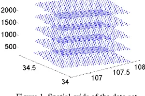
The data set is generated by the rigorous model of SPOT-5 HRS imagery. The original image size is 12000×12000 pixels. The elevation of the spatial grids varies from 200 to 200m. There are totally five layers with 500m height interval for control and check points. As shown in Fig 1. There are 552 image points evenly distributed in the image plane. The even points are used for control points, and the odd are check points. A spatial ray can be determined for image point by the projection centre and its image coordinate. The corresponding spatial coordinate of an image point can be calculated by intersection between the ray and a level plane with known elevation.
Figure 1. Spatial grids of the data set
3.2 Results of stepwise and orthogonal distance regression
The accuracy of the calculated RFM parameters directly influences the possible application of HRS imagery. In order to evaluate the accuracy computed by the proposed stepwise and orthogonal distance regression strategy, the error statistics of the calculated RFM parameters for the two methods are compared
with each other. As shown in Table 2, the accuracy of the computed RFM parameters by the proposed ORFM is higher than least squares and traditional orthogonal distance regression in cross-track (sample). In spite of lower accuracy in along-track, the proposed ORFM is more accurate and advantageous in sample and along than any least squares or orthogonal distance regression. Without the expense of accuracy, adopting stepwise selection to address the over-parameterization problem, in some extent, it can make the RFM parameters more sense. The numbers of RFM parameters in different methods is shown in Table 1.
Figure 2. Residues distribution of Least Squares
Figure 3. Residues distribution of Orthogonal Distance regression
Figure 4. Residues distribution of Stepwise and Orthogonal Distance regression
And the Fig 2, Fig 3, and Fig 4 show residues of RFM computed by least squares, orthogonal distance regression, and stepwise selection and orthogonal distance regression, respectively. All of the three have been optimized by Fourier series. The residues distribution and the Fourier series fitting in cross-track and along-track direction is showing as Fig 5 and Fig 6, respectively. These results show that the proposed ORFM can solve the over-parameterization and over-correction problem simultaneously.
Table 1. Numbers of RFM parameters of different methods
methods numbers of RFM parameters
Cross track Along track
Least Squares 39 39
Orthogonal Distance Regression 39 39
Figure 5. Fourier series fitting and residues in cross-track direction
Figure 6. Fourier series fitting and residues in along-track direction
Table 2. Accuracy of RFM computation (pixels)
Statistics items Least Squares Orthogonal distance
regression
The proposed ORFM
Cross track(Sample)
Maximum residues 1.037427 1.073696 1.027079
Root mean square error 0.016510 0.028758 0.014834
Along track(Line) Maximum residues 1.004564 0.987918 1.010222
Root mean square error 0.005182 0.006979 0.006881
Sample and Line Root mean square error 0.017304 0.029593 0.016352 4. CONCLUSIONS
A novel method for RFM parameter optimization by stepwise selection and orthogonal distance regression of settling over-parameterization and over-correction has been proposed. The proposed ORFM can fit the rigorous sensor model of HRS imagery with the least essential parameters and rational observation error, and thus, the ill-posed problem of RFM parameter estimation caused by over-parameterization and the over-correct of constant term are significantly alleviated. The experiments results show that more accurate can be obtained by the proposed method with only 37 essential parameters compared to least square and orthogonal distance regression with 78 parameters.
After optimized by a systematic error correction model with Fourier, the achieved RMSE of the proposed method is 0.014834 pixel and 0.006881 pixel for the cross track and along track directions, respectively. And the RMSE 0.016352 in across-track and along-track plane.
However, although the RMSE of proposed ORFM in cross and along plane is lowest, the RMSE in along direction is more inaccurate than least square, which indicates that there are still systematic residues in the along-track direction. Further investigation is planned to achieve more consistent results against the rigorous sensor model.
ACKNOWLEDGEMENTS
The authors thank National Natural Science Foundation of China (NSFC) (grant nos. 41101407), the Natural Science Foundation of Hubei Province (grant nos. 2014CFB377 and 2010CDZ005), China, and the self-determined research funds of CCNU from the colleges’ basic research and operation of MOE (grant nos. CCNU15A02001) for supporting this work. We are grateful for the comments and contributions of the anonymous reviewers and the members of the editorial team, especially Prof. Dr. Konrad Schindler.
REFERENCES
Carroll, R. J. and D. Ruppert,J., 1996. The Use and Misuse of Orthogonal Regression in Linear Errors-in-Variables Models. The American Statistician 50(1), pp.1-6.
Fraser, C. S. and H. B. Hanley,J., 2003. Bias compensation in rational functions for IKONOS satellite imagery. Photogrammetric Engineering & Remote Sensing 69(1), pp.53-57.
Goldberger, A. S. and D. B. Jochems,J., 1961. Note on Stepwise Least Squares. Journal of the American Statistical Association 56(293), pp.105-110.
Hu, Y. and C. V. Tao,J., 2002. Updating solutions of the rational function model using additional control information. Photogrammetric engineering and remote sensing 68(7), pp.715-724.
Jacobsen, K.,J., 2004. Use of very high resolution satellite imagery. Archiwum Fotogrametrii, Kartografii i Teledetekcji 14. Peiliang, X., L. Jingnan and S. Chuang,J., 2012. Total least squares adjustment in partial errors-in-variables models: algorithm and statistical analysis. Journal of Geodesy 86(8), pp.661-675.
Pope, P. and J. Webster,J., 1972. The use of an F-statistic in stepwise regression procedures. Technometrics 14(2), pp.327-340.
Tao, C. V. and Y. Hu,J., 2001. A comprehensive study of the rational function model for photogrammetric processing. Photogrammetric engineering and remote sensing 67(12), pp.1347-1358.
Topan, H., T. Taskanat and A. Cam,J., 2013. Georeferencing accuracy assessment of Pléiades 1A images using rational function model. International Archives of the Photogrammetry, Remote Sensing and Spatial Information Sciences 7, pp.W2. Wallace, T. D.,J., 1964. Efficiencies for Stepwise Regressions. Journal of the American Statistical Association 59(308), pp.1179-1182.
Y., J., Z. G., C. P., L. D., T. X. and H. W.,J., 2015. Systematic Error Compensation Based on a Rational Function Model for Ziyuan1-02C. IEEE Transactions on Geoscience and Remote Sensing 53(7), pp.3985-3995.