Directory UMM :Data Elmu:jurnal:I:International Review of Economics And Finance:Vol9.Issue4.2000:

(1)

International Review of Economics and Finance 9 (2000) 323–350

Choice of currency basket weights and its implications

on trade balance

Hsiang-Ling Han*

Economics Division, Babson College, Wellesley, MA 02457-0310, USA

Received 14 August 1998; revised 10 June 1999; accepted 23 August 1999

Abstract

This paper seeks to find an optimal choice of currency basket weights for emerging econo-mies that peg their currencies to a currency basket, and to examine the long-run relationship between the real exchange rates of a group of trading partners. A general equilibrium model is set up to establish an optimal set of currency basket weights, coupled with the choice of fiscal policy, tosimultaneouslystabilize trade balance and aggregate price level of an economy. This optimal set of weights is a weighted average of two sets of weights; each targets at one policy goal (stabilizing either balance of trade or aggregate price level) at a time. Empirical studies including vector autoregression (VAR) analysis and cointegration analysis on the long-run relationship between the Thai baht and the real exchange rates of its major trading partners are presented. 2000 Elsevier Science Inc. All rights reserved.

JEL classification:F31; C32

Keywords:Currency basket; Vector autoregression; Cointegration

1. Introduction

The Dow Jones Industrial Average lost more than 7 percent of its value on October 28, 1997. It was preceded by a 5.8 percent plunge in the Hong Kong Stock Market following months of speculation and devaluation of Southeast Asian currencies. Many people believe that the downward spiral originated in the Thai government’s insistence on pegging the Thai baht to the U.S. dollar. The domino effect eventually reached South Korea and Japan. South Korea’s currency, the won, lost the maximum daily trading limit, 10 percent of its value, on November 20, 1997. The demise of a powerful Japanese broker, Yamaichi Securities Co., on November 24, 1997, propelled the Asian currency and financial crises to another climax.

* Corresponding author. Tel.: 781-239-5851; fax: 781-239-5239.

E-mail address: [email protected] (H.-L. Han)

(2)

The debate on the optimal exchange rate policy that prevents this type of financial crisis from happening has been going on for decades. The focus of this paper, however, is on the choice of currency basket weights and its implications on trade balance for emerging economies. It is known that most of the Southeast Asian countries that encounter currency crises peg their currency to a basket dominated by the U.S. dollar. The paper, using Thailand as an example, investigates whether the choice of currency basket weights is optimal and the relation of the currency basket weights with its balance of trade.

A general equilibrium model is set up to establish an optimal choice of currency basket weights, coupled with an optimal fiscal policy, to simultaneously stabilize overall balance of trade and price level of an economy. The model takes multilateral trade flows as well as macroeconomic policy targets into consideration. Long-run relation-ships between the Thai baht and the real exchange rates of its major trading partners are then explored. Thailand is used to conduct the empirical work of the paper because it is believed that this wave of currency crisis was originated there. It is interesting to analyze and to examine how the currency basket weights chosen by the Thai government affect the value of the Thai baht, their trade balance, and their current account balance, even though those weights are not officially publicized.

Two approaches are used to analyze the long-run relationships between the Thai baht and the real exchange rates of its major trading partners. Vector autoregression (VAR) analysis is used to estimate a system of interrelated real exchange rates and to analyze the dynamic impact of random disturbances on the system of variables. The impulse-response function is presented to trace the effect of a shock to a real exchange rate on current and future values of another real exchange rate. The second approach, focusing on the long-run cointegrating relationship between these real exchange rates, includes canonical cointegrating regression (CCR) and Johansen’s LR test.

Most tests for cointegration [e.g., Engle & Granger (1987) and Phillips & Ouliaris (1988)] took the null hypothesis of no cointegration. Failures to reject the null hypothesis of no cointegration are often interpreted as evidence against economic models thaty cointegration. This type of methodology is known to have relatively low power. The two methodologies used in this paper, however, are relatively powerful and have good small sample properties. CCR proposed by Park (1992) tests the null hypothesis of cointegration. Han (1996) investigated the small sample properties of the CCR tests and concluded the tests perform well with reasonable size and power even when the samples are small. The Johansen’s LR test is now commonly used, and numerous researches have proven it to be a reasonable testing method for cointegration.

(3)

first set of results includes a vector autoregression (VAR), variance decomposition, and impulse-response function analysis. The second set of results includes the test for cointegration and the estimation of cointegrating vector for the group of currencies. Section 6 is the concluding remarks.

2. Literature review

Most of the literature relating to the choice of exchange rate arrangements is cast in terms of a dichotomy between fixed and flexible exchange rates. In practice, however, systems of rigidly fixed or perfectly flexible rates are hardly ever observed. Different types of exchange rates arrangements may be appropriate for different countries, de-pending on their structural characteristics, external environments, and macroeconomic and political circumstances. Moreover, as structural characteristics, external environ-ments, or macroeconomic and political circumstances change over time, market pres-sures on exchange rates may sometimes become so overwhelming that they essentially force changes in the exchange rate arrangements (like what happened in Thailand). Discussions of optimal currency arrangements have changed considerably over the past half-century. The debate over fixed versus flexible exchange rates around 1960 centered on the issue of whether international capital flows would be stabilized under flexible rates (Friedman, 1953). A new school of thought emerged in 1960s, analyzing the types of structural characteristics that made it optimal for a country to choose one type of arrangement over the other (Mundell, 1969; McKinnon, 1963; Kenen, 1969). These studies focused on a number of relevant structural characteristics of economies, including size and openness, diversity of production activities and occupa-tional skills, geographic factor mobility, fiscal redistribution mechanisms, policy prefer-ences, wage and price flexibility, exposure to shocks, and level of financial develop-ment. Mundell also led the analysis of optimal currency areas. He defined an optimal currency area as “a domain within which exchange rates are fixed,” rather than an area with a single currency.

The conventional wisdom in the 1970s was that the currencies of developed countries should float but the currencies of less-developed countries (LDCs) should not. With the advent of generalized floating, both Malaysia and Singapore allowed their currencies to float until both countries decided in 1975 to peg their currencies to baskets of currencies of their trading partners. Korea and Thailand initially pegged their currencies to the U.S. dollar, but later switched to pegging their currencies to basket composites after a major devaluation of the nominal exchange rates. Korea switched from the dollar peg to the composite peg in 1980 following a 20-percent devaluation, while Thailand adopted the basket pegging arrangement after a devaluation in 1985. The Philippines officially adopted the U.S. dollar peg system, while making several adjustments to the nominal parity through a series of devaluations (Gan, 1994).

(4)

the scope for international policy cooperation, and the endogeneity of factor mobility or other structural characteristics (Edison & Melvin, 1990). By the mid-1980s, the policy-making community actively discussed proposals for replacing the system of flexible exchange rates among major currencies with a system of target zones (Krug-man, 1991). A “target zone” is an arrangement with wide margins around an adjustable set of exchange rates. In early 1990s, the theory of optimal currency areas was to consider various practical issues associated with the move toward monetary integration in Europe (Bayoumi, 1994).

More recently, the study on exchange rate regimes is linked with financial fragility and macroeconomic policies. Chang and Velasco (1997) found that a currency board cannot implement a socially optimal allocation. In addition, bank runs are possible under a currency board. They also found that a fixed exchange rate system may implement a social optimum but is more prone to bank runs and exchange rate crises than a currency board. However, they found that a flexible exchange rate system implements the social optimum and eliminates runs, provided the exchange rate and central bank lending policies are appropriately designed.

The focus of this paper is to search for explanations for the 1997 Asian foreign exchange market crises. Therefore, only the currency basket arrangement that has been adopted by most of the Southeast Asian countries is studied here. One explanation is that the choices of weights to determine basket composites of these countries may not be adequate to deter speculators from attacking these Southeast Asian currencies. For example, the top priority of the central bank of Thailand for the period of 1985 to 1997 has been to hold the baht stable against a basket of currencies dominated by the U.S. dollar. The policy helped to cut inflationary expectations in Thailand and made it one of the world’s fastest-growing economies, but also created a huge current account deficit. The inter-relationship between currency basket weights, overall trade balances, and price level will be analyzed in our model.

3. The basic model

The model is set up to show that a combination of optimal fiscal policy and currency basket weights can reach two policy goals at the same time (e.g., keep the overall balance of trade as well as price level unchanged). The analysis is based on Branson and Katseli (1981), and can be extended to include other economic policies such as monetary policy and trade (tariff) policy.

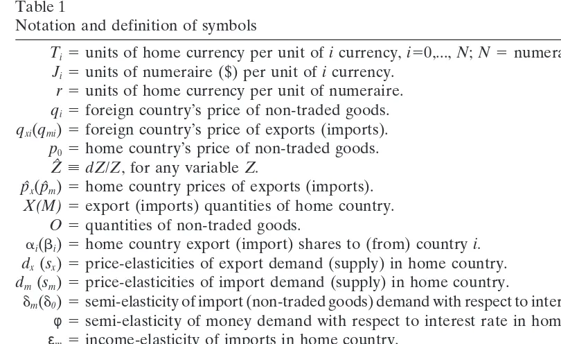
Assume that the home country produces two goods: exports goods and nontraded goods. Exports are not consumed by the home country residents and nontraded goods are consumed only by the home country residents. The real exchange rate stabilization is also assumed in the model as in Branson and Katseli (1981). Notation and definition of the symbols used in the model are summarized in Table 1.

3.1. The export market

(5)

Table 1

Notation and definition of symbols

Ti5units of home currency per unit oficurrency,i50,...,N;N5numeraire country.

Ji5units of numeraire ($) per unit oficurrency.

r5units of home currency per unit of numeraire.

qi5foreign country’s price of non-traded goods.

qxi(qmi)5foreign country’s price of exports (imports).

p05home country’s price of non-traded goods.

Zˆ ;dZ/Z, for any variableZ.

pˆx(pˆm)5home country prices of exports (imports).

X(M)5export (imports) quantities of home country.

O5quantities of non-traded goods.

ai(bi)5home country export (import) shares to (from) countryi.

dx(sx)5price-elasticities of export demand (supply) in home country.

dm(sm)5price-elasticities of import demand (supply) in home country.

dm(d0)5semi-elasticity of import (non-traded goods) demand with respect to interest rate in home country.

φ5semi-elasticity of money demand with respect to interest rate in home country. εm5income-elasticity of imports in home country.

ε05income-elasticity of non-traded goods in home country.

u 5share of non-traded goods spending to total spending in home country.

BT5balance of trade on goods and services in home country’s currency.

MY5quantity of money.

R5domestic nominal interest rate.

y05real income of home country.

The export supply function can be written as shown in Eq. (1),

lnX5 sx(lnpx2lnp0), (1)

which implies that the higher relative price of exports to nontraded goods, the more exports will be supplied.

Demand for the home country exports by countryi, given countryi’s currency price of the home country exports and country i’s currency price of its own nontraded goods, is specified as shown in Eq. (2):

lnXi5 2dx(lnqxi2 lnqi). (2)

That is, the home country export demand by countryi is a function of the relative price of the home country exports (countryi’s imports) to countryi’snontraded goods (qxi/qi), both measured in countryi’s currency. The price elasticity of export demand

in all countries is assumed equal dx to for simplicity. Goods arbitrage ensures the

equality of the home country currency price of exports (px) and country i’s currency

price of exports (Tiqxi), as shown in Eq. (3),

px5Tiqxi, (3)

whereTi;Jir.

(6)

Total differentiation of the condition shows that percentage change in export price (pˆx) is a function of percentage change in the price of domestic nontraded goods (pˆ0),

percentage change in the home country’s real exchange rate against the numeraire, (rˆ 1qˆN 2pˆ0), as well as percentage change in the numeraire’s real exchange rates

against third countries, (Jˆi1qˆi2qˆN), as shown in Eq. (4),

pˆx5pˆ01k(rˆ 1qˆN 2pˆ0)1 k

o

ai(Jˆi1qˆi2qˆN), (4)

wherek ;dx/(dx1sx).

As mentioned in Branson and Katseli (1981), k represents market power on the export (the home country) side. A small country assumption meansk51. By substitut-ing condition (4) into the export market (1), Eq. (5) can be shown:

Xˆ 5sxk([rˆ 1qˆN 2pˆ0) 1

o

ai(Jˆi1qˆi2 qˆN)]. (5)

Percentage change in exports is a function of percentage change in the home country’s real exchange rate, percentage change in foreign real exchange rates, and the parame-ters ofkand sx.

3.2. The import market

In the import market, assume that the home country government spends aG on imports, where Gindicates the government spending and a indicates the portion of government spending on imports. The supply of imports by countryiis a function of the relativei-currency price of imports (i.e., countryi’s exports) to countryi’s nontraded goods. It is similar to Eq. (1) and it can be expressed as shown in Eq. (6):

lnMi5sm(lnqmi 2lnqi). (6)

The aggregate demand for imports by the home country is dependent on the relative home currency price of imports to nontraded goods, the real income level, the nominal interest rate, and the government spending in the home country, as shown in Eq. (7),

lnM 5 2dm(lnpm2lnp0) 1εmlny2 dmR 1 gmlnG, (7)

wheregm5aG/Mindicates the government spending share of imports market.

Equat-ing the demand and supply of imports, it is shown that the correspondEquat-ing change in the import price is a function of percentage change in the price of domestic nontraded goods, percentage change in the home country’s real exchange rate, percentage change in foreign real exchange rates, percentage change in the real income, change in the nominal interest rate, government spending, and other elasticity parameters. Eq. (8) is given as follows:

pˆm5pˆ01k9(rˆ 1qˆN2pˆ0) 1k9

o

bi(Jˆi 1qˆi2qˆN) 1ε9myˆ 2 d9mdR1 g9mGˆ,

(8)

wherek9 ;sm/(dm1sm),d9m;dm/(dm1sm),ε9m;εm/(dm1sm), andg9m;gm/(dm1sm).

(7)

3.3. The nontraded goods market

Demand and supply of nontraded goods for the home country are specified in an analogous way. Percentage change in the price of nontraded goods can be expressed as shown in Eq. (9),

pˆ05k0pˆx1(12k0)pˆm 1ε90yˆ 2 d90dR 1 g90Gˆ, (9)

wherek0;s0/(s01d0),ε90 ;ε0/(s01d0), d90;d0/(s01d0),g90 ;g0/(s01d0), andg0;

(1 2 a)G/O is the government spending share of nontraded goods. Eq. (9) means that percentage change in the price of nontraded goods is dependent on percentage change in the price of exports and imports, percentage change in the real income, change in the nominal interest rate, and percentage change in the government spending. It can also be shown that percentage change in nontraded goods (Oˆ) depends on the same factors that affect percentage change in the price of nontraded goods.

3.4. The money market

Demand for real money balances is a function of the real income and the nominal interest rate, as shown in Eq. (10),

lnMY 2lnpI5lny 2φR, (10)

wherepIis the consumer price index (CPI) and is defined asCPI 5pI5pu0 p(1m2u). It

is assumed that the interest rate (R) can be chosen by the central bank to certain extent. For example, the Bank of Thailand (BOT) successfully adjusted the interest rate ceiling and monitored credits extended to the private sectors in early 1980s. From 1985 to 1985, the BOT also played a leading role in bringing down domestic interest rates by reducing interest rate ceilings on several occasions. Let us focus on the impacts of fiscal policy, and assume that there is no tariff and no monetary policy (Mˆ Y 50). The real income of the home country is defined as the nominal income divided by the aggregate price level, as given by Eq. (11):

y 5p0O1pxX

pu

0 p(1m2u)

. (11)

Differentiating both sides of Eq. (11) gives Eq. (12):

yˆ 5a(pˆ01Oˆ) 1b(pˆx1Xˆ) 2 upˆ02 (12 u)pˆm, (12)

wherea 5p0O/(p0O 1pxX), b5 pxX/(p0O1pxX), anda 1 b5 1. Substituting all

percentage changes of nontraded goods, price of nontraded goods, exports, price of exports, and price of imports (pˆ0,Oˆ,pˆx,Xˆ,pˆm) into Eq. (12), it can be shown that,

according to Eq. (13):

yˆ 5(a(11s0) 2bsx)pˆ01(b(11sx) 2as0)pˆx2 u pˆ02(12 u)pˆm

5Apˆ01 Bpˆx2 upˆ02(1 2 u)pˆm, (13)

whereA5a(11s0)2bsx, B 5b(11sx) 2as0,A1B51 andA.0, B.0. Eq.

(8)

changes in all prices, including nontraded goods, exports, and imports. Then, substitut-ing percentage change in the real income (yˆ) into Eq. (10) and lettsubstitut-ing Mˆ Y 5 0, it shows that change in the nominal interest rate is as shown in Eq. (14):

dR51

φ(Apˆ01Bpˆx). (14)

When the prices of nontraded goods and exports increase, the nominal interest rate increases.

Next is to solve the simultaneous equations of (4), (8) and (9) forpˆx,pˆm,pˆ0and then

forXˆ,Mˆ ,Oˆ. These results will further be utilized to determine the optimal weights for different policy goals. Details are shown in mathematical appendix.

3.5. Policy goals

3.5.1. Stabilizing the balance of trade

The balance of trade on goods and services in the home country currency is defined asBT5pxX2pmM.DifferentiatingBTand choosingpx5pm51 initially result in

Eq. (15):

dBT5(pˆx1Xˆ)X2 (pˆm1Mˆ )M. (15)

Substituting the results from previous section onpˆx,pˆm,Xˆ,Mˆ and assuming thatX5M

at the beginning leads to Eq. (16),

dBT5 G1pˆ01 G2pˆx1 G3pˆm2 gmGˆ, (16)

where G1 5 2(sx 1 dm) 2 (εm2 dm/φ)A 1 εmu, G2 5 (1 1 sx) 2 (εm 2 dm/φ)B, and G35 2(12 dm) 1 εm(12 u). Substitutingpˆ0,pˆx,pˆm(see the appendix) into Eq. (16),

we get Eq. (17),

dBT5H1(rˆ 1qˆN 2pˆ0) 1

o

H2i(Jˆi1qˆi2 qˆN) 1H3Gˆ, (17)

whereH15 G1E11 G2P11 G3L1, H2i 5 G1E2i 1 G2P2i 1 G3L2i, H3 5 G1E31 G2P3 1

G3L32 gm. The detailed definition of E1, E2i, E3, P1,P2i, P3,L1,L2i,L3, can be found

in the mathematical appendix. If

(sx1 dm) 1(εm2 dm/φ)A

εm

, u ,εm2(12 dm)

εm

it can be shown thatG1,G2,G3are positive, thereforeH1andH2iare positive. But the

sign for H3is uncertain and depends on the government spending share of imports

(gm). To stabilize the trade balance and letdBT50, the home country’s real exchange

rate against the numeraire must equal, as shown in Eq. (18):

(rˆ 1qˆN 2pˆ0) 5 2

o

wi(Jˆi 1qˆi2qˆN) 2Z1Gˆ, (18)

where the weight is defined as H21

1 H2i and is the weight in a currency basket if the

balance of trade is kept unchanged, andZ1, defined as H211H3, is the reaction of the

(9)

(Jˆi1qˆi2qˆN) (i.e., the depreciation ofith currency), will deteriorate the trade balance

byH2i. In order to keep the balance of trade unchanged and to offset the impact from

the depreciation ofith currency, the home country currency against numeraire (rˆ 1

qˆN2pˆ0) should increase (depreciate) according towi. Also, when government spends

more on imports, the trade balance will deteriorate and the home currency should depreciate according toZ1.

Branson and Katseli (1981) show that the weights to be chosen in a currency basket in order to stabilize real exchange rate, without including any policy variable to reach any policy goal, is (rˆ1 qˆN2 pˆ0) 5 2

o

wBKi (Jˆi1 qˆi2qˆN) Stabilization of real

ex-change rate is also assumed in our model. However, in contrast to Branson and Katseli’s (1981) model, we include the policy variable (G) in Eqs. (7), (8), (9), and consider a nontraded market affected by government purchases (G). Eq. (18) is derived following these assumptions. Eq. (18) indicates that government purchases could change and the home country currency against numeraire (rˆ1qˆN2pˆ0) should react

to the change according to Z1, even though the real value of ith currency does not

change. The termviin Eq. (18) is the weight in a currency basket if we want to keep the trade balance unchanged. The term Z1 in Eq. (18) is the optimal exchange rate

response to an exogenous change in government purchases if we want to keep the trade balance unchanged. Both are derived under the assumptions stated in the model.

3.5.2. Stabilizing the consumer price index

The consumer price index is defined in the previous section as CPI 5 pI 5

pu

0p(1m2u). Therefore, the change in the CPI is pˆI5 upˆ0 1 (12 u)pˆm. LettingpˆI5 0,

Eq. (19) can be shown,

(rˆ 1qˆN 2pˆ0)5 2

o

w9i(Jˆi1 qˆi2qˆN) 2Z2Gˆ, (19)

wherew9i 5(uE11(12 u)L1)21(uE2i1(12 u)L2i) andZ25(uE11(12 u)L1)21(uE31

(12 u)L3). Both can be shown to be positive. In order to keep the CPI unchanged,

whenith currency appreciates [(Jˆi1qˆi2 qˆN) increases], the home country currency

against numeraire, (rˆ1qˆN2pˆ0), should appreciate (decrease) according tow9i. When

the government purchases increase by one percent, the home country currency should appreciate according toZ2, even though the real value ofith currency does not change.

Eqs. (18) and (19) give us the weights in a currency basket if we are aiming at either stabilizing balance of tradeorconsumer price index. As clearly shown in these equations, it is possible for the government to optimally implement both fiscal policy and currency basket policy to stabilize balance of trade and consumer price index simultaneously.

3.5.3. Stabilizing both the balance of trade and the consumer price index

To show the case that changes in the balance of trade and the consumer price index are zero simultaneously, one need to combine Eqs. (18) and (19) into Eq. (20),

(rˆ 1qˆN 2pˆ0)5 2

o

wi(Jˆi1 qˆi2qˆN) 2Z1Gˆ 5 2

o

w9i(Jˆi1qˆi2qˆN) 2Z2Gˆ,

(20)

(10)

Gˆ 5

o

w9i 2wi

Z12Z2

(Jˆi1qˆi 2qˆN). (21)

In order to stabilize both the over all trade balance and the consumer price index, government purchase (G) is no longer an exogenous variable and should follow the process as specified in (21). G has to respond to a change in the real value of ith currency. We then substitute Eq. (21) into Eq. (17) to get Eq. (22),

(rˆ 1qˆN 2qˆ0) 5 2

o

[rw9i 1(12 r)wi](Jˆi1qˆi2qˆN) 5 2

o

w*i (Jˆi1qˆi2qˆN),

(22)

wherer 5 Z1

Z12Z2

.

From Eqs. (21) and (22), it is shown that both G and the home country currency (rˆ1qˆN2pˆ0) have to respond to the changes in the real value ofith currency at (Jˆi1

qˆ12qˆN) the same time to stabilize overall balance of trade and consumer price index.

The optimal weight in a currency basket (w*) that reaches these two policy goals simultaneously is a weighted average of two separate sets of weights (wi,w9i), each

targeted at one policy goal. The weight r is a function of the structural parameters. The results show that by combining an optimal fiscal policy that follows Eq. (21) with a currency basket peg that uses an optimal set of weights [w* in Eq. (22)], one economy can insulate its overall balance of trade and aggregate price level from a change in a third-country’s real exchange rate.

4. The currency basket system in Thailand

To understand the evolution of the exchange rate policy in Thailand, one has to analyze the macroeconomic performance during the period of 1980 to 1997. From 1980 to 1984, Thailand experienced a number of economic problems as the result of an unfavorable world economic environment and, to a certain extent, of domestic overspending. The major problem encountered during this period was the threat of external instability. The problem of external imbalance became most serious in 1983 when the current account deficit reached 7 percent of GDP, international reserves dwindled to only three months imports, and the external debt level increased rapidly. With this in mind, demand-management policy during this period was aimed at reduc-ing external imbalance towards a sustainable level. As a consequence of these stabiliza-tion policies coupled with a weak world economic environment, real economic growth slowed down to an annual average of 5 percent by the mid-1980s.

(11)

externally, economic growth was weak. Real GDP had a growth rate of slightly more than 3 percent in the 1985–86 period.

The policy focus during the 1985–1986 period was therefore shifted towards stimulat-ing a recovery of the economy. By 1987, the economic growth had been revived. Particularly, Thailand experienced an economic boom during the period 1987–1990, characterized by an average rate of economic growth of over 10 percent a year. This record of economic growth is regarded as being exceptionally high both in absolute terms and in comparison with other dynamic countries in the entire Asia-Pacific region [see e.g., Robinson, et al. (1991), p. 10, and Asian Development Bank (1992)]. The double-digit growth rates were accompanied by modest, though increasing, domestic inflation rates (2.5–6.0 percent annually). In addition, current account deficits were kept at an average of around 4 percent of GDP, while international reserves and the external debt position became healthier than during the earlier period.

The monetary and exchange rate policies from 1980 to 1997 are closely related to the above-mentioned macroeconomic performance. Discretionary, restrictive fiscal and monetary policies as well as exchange rate management were implemented and monitored with great caution to restore economic stability. Regarding fiscal policy, the government put much effort into curbing the growth of its expenditure and into increasing its efficiency in revenue collection. On the monetary policy front, a high interest rate policy was adopted with the aim of achieving three objectives. One was to induce more domestic savings, another was to slow down credit expansion, and the last one was to align domestic with foreign interest rates in order to prevent capital outflow.

In this connection, the Bank of Thailand (BOT) successively adjusted interest rate ceilings and monitored credits extended to the private sector, particularly those for import purposes. These measures, combined with other anti-inflationary measures launched by several government agencies, were, to a large extent, successful in reviving internal stability by bringing down the inflation rate from 19.9 percent in 1980 to 3.8 percent in 1983. In contrast, external instability was still left unresolved. Eventually, in January 1984, a tighter measure of monetary policy, direct credit control, was imposed on domestic commercial banks to reduce the rapid expansion of credit. The use of this measure was regarded as a new experience for Thailand’s monetary management at the time. This measure was, however, abolished eight months later as it was claimed in some circles as being too restrictive in bringing down the credit expansion [Akrasanee, et al. (1991)].

As for the arrangement for the Thai baht, it can be divided into five distinct phases: (1) the pre-par value system (until 1963); (2) the par value system (1963–1978); (3) the daily fixed system (1978–1981); (4) the de facto fixed system (1981–1984); and (5) the basket of currency system (1984– present). The focus of this paper is more on the last two periods.

(12)

by 1.1 percent in May and the second time by 8.7 percent in July. At the same time, the daily fixing system between the Thai baht and the U.S. dollar was replaced by a fixed exchange rate system. Although the devaluation of the baht had to a certain extent helped improve Thailand’s external balances, its beneficial effects were short-lived due to the prolonged strength of the U.S. dollar.

The Thai baht was devalued once again by 14.8 percent in November 1984, shortly after the credit control scheme was revamped, and since then the value of the Thai baht has been pegged to a basket of currencies. The move to this new exchange rate system was viewed as an important step toward the use of a more flexible exchange rate regime. At the very beginning of adopting this system, the Thai baht was pegged to a basket of the currencies of Thailand’s major trading partners. The weighting scheme at that time was based on the relative importance of the currencies of Thailand’s trading partners. Detailed information of this weighting was not publicized, and that provided the monetary authorities some discretion in the implementation of exchange rate policy.

This kind of weighting scheme was used for about one year. After the G-7 meeting in September 1985 and the currency realignment, the U.S. dollar depreciated rapidly. This led the Thai authorities to adjust the weighting scheme by giving a higher weight to the U.S. dollar, from approximately 50–55 percent to 80–85 percent [Akrasenee, et al. (1991), p. 239]. The actual weights of currency basket, however, continue to be not publicized. In this regard, exchange rate policy has been claimed to be an important instrument in correcting external disequilibrium problems in Thailand over the period 1980–1991. As documented in Wibulswasdi (1987 and 1988), the main focus of the exchange rate policy in Thailand has been to support the competitiveness of exports while maintaining the confidence of participants in the exchange market. Subsequent developments in the financial and economic conditions of the country proved that the implementation of the new exchange rate policy achieved the intended objectives up to 1996.

Under the new exchange rate regime, the baht-U.S. dollar rate is the exchange rate that has been used by the monetary authorities as a basis for setting an appropriate level for the baht’s external value against other major trading partners [e.g., Japan, the U.K., Germany, Hong Kong, Malaysia, and Singapore; see Hataiseree (1995)]. More precisely, such a nominal exchange rate is set by the Exchange Equalization Funds (EEF) Committee. This committee was created by a special law in 1955 with a mandate to stabilize and maintain the external value of the Thai baht at a level deemed appropriate for domestic overall economic and financial conditions. Although the EEF is legally set up as a separate entity from the BOT, its top executive personnel have always come from present high-ranking officials at the BOT to ensure a close collaboration between the two institutions.1

(13)

(1988), pp. 13–15]. Since the adjustments based on (1) and (2) have generally been regarded as short-run in nature, their effects on the rate setting seem to be minimal. Nevertheless, adjustments in the exchange rate following developments in these two factors have to be pursued constantly in order to shield the domestic economy from the adverse effects of fluctuations in the exchange rates of major currencies in the international foreign exchange market.

Adjustments of the exchange rate based on (3) have been viewed as being the most important, since they constitute a policy intention of the BOT. Intervention actions under this last category are primarily aimed at addressing a broader issue of Thailand’s economy over a longer period, such as a deterioration in competitiveness, external debt, or the balance of payments.

However, all three of these types of adjustments started to show their lack of control over the Thai economy in late 1996. Under the currency basket since 1985, the Thai baht has been determined overwhelmingly by the U.S. dollar. However, at the same time, Thailand had and continues to have substantial trade relationships with Japan. As the Japanese yen depreciated against the U.S. dollar from April 1995 to the summer of 1997, the real effective exchange rate of Thai baht appreciated against the Japanese yen. Due to the appreciation, export competitiveness was lost. Export from Thailand declined and current account deficits increased in the 1996–1997 period. This currency basket system therefore became the prime force that triggered the Asian currency crisis.

5. The long-run relationship between real exchange rates

The long-run relationship between real exchange rates of a group of trading partners, when the balance of trade is kept unchanged, is implied in Eq. (18). It shows that, in order to stabilize the trade balance of the home country, whenith currency against the numeraire depreciates by 1 percent, the home currency against the numeraire should also depreciate by vi% to maintain the relative competitiveness. The total

impact from all currencies in the basket on the value of the home currency should add up to one. The results can be used to test the overall competitiveness of the home country and to analyze the effect of exchange rate movement of the home country on its trade balance. Because the actual weights employed by the BOT are not known to the public, it is not appropriate to directly compare the optimal weights derived from the model and the actual weights used in the Thai currency basket. However, there are other methods to analyze how far apart the used weights were from the optimal weights and their implications on trade balances.

The nonstructural approach of vector autoregression (VAR) is first applied to estimate the response of the home country currency when the values of its trading partners’ currencies depreciate or appreciate. The VAR results are further examined to assess the cause of trade balance surplus or deficit in the home country. The impulse response analysis and variance decomposition are also performed.

(14)

to a basket, there should be a long-run relationship between the log levels of the real exchange rates (all measured against the numeraire) of countries involved. It means that the percentage change in the real exchange rates among trading partners should be cointegrated. Analyzing the cointegrating vector will also shed new light on whether or not the used weights are optimal.

The augmented Dickey-Fuller test is applied to test the nonstationarity of the log levels of real exchange rates prior to perform cointegration tests. Johansen’s LR test and the canonical cointegrating regression proposed by Park (1992) are then used to test for cointegration and to estimate the cointegrating vector.

After normalizing the cointegrating vector (1,2b1,2b2,...,2bi)9, it is implied in the

model that, if the trade balance of the home country is stabilized, the summation of the elements in the cointegrating vector ought to be zero. That is, the summation of the impact of all the currencies in the basket is negative one. If the summation of the elements in the cointegrating vector is negative, the percentage change in the home country’s real exchange rate is less than the uniform percentage change in its trading partners’ real exchange rates. It indicates that the home country currency is relatively inflexible, comparing to the currencies chosen in its currency basket. The inflexibility will affect the home country’s competitiveness in the exports market. It may also cause international speculative attacks on the home currency.

5.1. Vector autoregression (VAR)

Assume all the real exchange rates in a currency basket are endogenous variables, and every endogenous variable in the system is a function of the lagged values of all the endogenous variables in the system. The VAR is expressed as shown in Eq. (23),

yt5A1yt211 A2yt211... 1Apyt2p 1Bxt1εt, (23)

whereytis ak 31 vector of endogenous variables,xtis ad 31 vector of exogenous

variables, A1, ..., Ap and B are matrices of coefficients to be estimated, and εt is a

vector of innovations that may be contemporaneously correlated with each other but are uncorrelated with their own lagged values and uncorrelated with all of the right-hand-side variables.

Following the estimation of an unrestricted VAR are the impulse response analysis and variance decomposition. An impulse response function traces the effect of a one standard deviation shock to one of the innovations on current and future values of the endogenous variables. By contrast, variance decomposition decomposes variation in an endogenous variable into the component shocks to the endogenous variables in the VAR. The variance decomposition gives information about the relative impor-tance of each random innovation to the variables in the VAR.

(15)

5.1.1. Data

The data are all quarterly, covering from 1981 Q1 to 1998 Q1 period. Bilateral real exchange rates are calculated using nominal exchange rates and consumer price indices (CPIs). The data are taken from the IMF’s International Financial Statistics; Board of Governors, Federal Reserves System; Bureau of Labor Statistics, Department of Labor; Statistics Bureau and Statistics Center, Management and Coordination Agency, Government of Japan; and Datastream International, Inc.

5.1.2. Empirical results on the VAR

Table 2 presents the VAR results. The AIC criterion is used to determine the lag periods. It is found that the log level of the Thai baht mainly depended on its own past values, which indicate the relative inflexibility of the Thai baht responding to changes in the currency values of its trading partners. The results also show that the log levels of the five real exchange rates are close to I(1) process. (Formal tests will be performed later.) It is also found that when the real exchange for the Japanese yen against the U.S. dollar increased (i.e., the Japanese yen depreciated), the real exchange rate for the Thai baht against the U.S. dollar decreased (i.e., the Thai baht appreciated). This would make Thai products be relatively uncompetitive, would lead to a trade deficit with Japan, and would cause an increase in the deficit of its current account. The same scenario would happen when the value of the Dutch Guilder changed. Yet the coefficient for the Dutch Guilder is not significant.

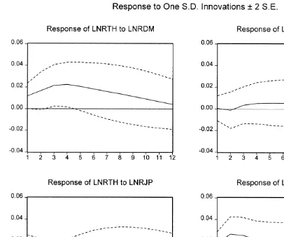
It is more interesting to examine the impulse response function and variance decom-position to see the actual response of the log level of Thai baht to the changes in the log levels of other currencies. The impulse response functions and variance decomposi-tion are calculated using the ordering: log DM, log Guilder, log yen, log Singapore dollar, and log baht. Four impulse response functions are plotted in Fig. 1, representing the effects of the first four innovations (to the log levels of DM, Guilder, yen, and Singapore dollar) on the log level of Thai baht.

It is observed that an increase in (a positive shock to) the log levels of Deutsche Mark and Singapore dollar was associated with an increase in the log level of Thai baht for the first two to three quarters, but this increase was reverse afterwards. Within about 12 quarters, the shock had almost disappeared. When the Deutsche Mark and the Singapore dollar depreciated, the Thai baht followed at first, but only lasted for about three quarters. If no other policy was implemented, Thai products would lose their relative competitiveness against German and Singaporean products by the end of third year.

(16)

→

/

International

Review

of

Economics

and

Finance

9

(2000)

323–350

LNRTH(21) 1.045469 (0.15194) (6.88073) 0.013519 (0.15341) (0.08812) 0.021640 (0.15632) (0.13843) 0.132609 (0.16982) (0.78086) 0.155962 (0.05890) (2.64810) LNRTH(22) 20.226498 (0.18752) (21.20787) 20.109533 (0.18934) (20.57851) 20.087936 (0.19293) (20.45580) 20.379279 (0.20959) (21.80964) 20.009704 (0.07269) (20.13350) LNRDM(21) 0.418811 (0.88636) (0.47251) 20.051967 (0.89494) (20.05807) 20.638529 (0.91193) (20.70020) 20.157715 (0.99068) (20.15920) 0.221411 (0.34357) (0.64444) LNRDM(22) 20.761059 (0.89325) (20.85201) 1.256538 (0.90190) (1.39321) 0.995377 (0.91902) (1.08309) 0.918662 (0.99838) (0.92015) 0.462185 (0.34624) (1.33485) LNRNH(21) 20.177908 (0.85156) (20.20892) 1.037346 (0.85981) (1.20648) 1.661087 (0.87613) (1.89594) 0.035256 (0.95178) (0.03704) 20.030009 (0.33008) (20.09091) LNRNH(22) 0.575499 (0.87798) (0.65548) 21.410117 (0.88649) (21.59068) 21.197253 (0.90331) (21.32541) 20.743117 (0.98131) (20.75727) 20.617504 (0.34033) (21.81445) LNRJP(21) 20.318936 (0.16616) (21.91947) 20.018446 (0.16777) (20.10995) 20.056266 (0.17095) (20.32914) 1.083948 (0.18571) (5.83664) 20.099323 (0.06441) (21.54212) LNRJP(22) 0.306752 (0.17089) (1.79500) 0.093927 (0.17255) (0.54435) 0.128707 (0.17582) (0.73203) 20.221109 (0.19100) (21.15761) 0.076590 (0.06624) (1.15621) LNRSP(21) 0.501686 (0.44691) (1.12257) 0.027178 (0.45124) (0.06023) 20.049290 (0.45980) (20.10720) 20.306825 (0.49950) (20.61426) 0.827253 (0.17323) (4.77542) LNRSP(22) 20.474563 (0.39467) (21.20242) 20.129407 (0.39850) (20.32474) 20.079578 (0.40606) (20.19598) 0.207487 (0.44112) (0.47036) 20.068937 (0.15298) (20.45062) C 0.552900 (0.64661) (0.85508) 0.126567 (0.65287) (0.19386) 0.088234 (0.66526) (0.13263) 1.572386 (0.72271) (2.17569) 20.167315 (0.25064) (20.66755)

R-squared 0.747573 0.919639 0.894297 0.946083 0.962938

Adj. R-squared 0.702497 0.905289 0.875422 0.936455 0.956320

Sum sq. resids 0.161343 0.164484 0.170785 0.201555 0.024242

S.E. equation 0.053676 0.054196 0.055224 0.059993 0.020806

Log likelihood 106.8999 106.2539 104.9945 99.44505 170.3973

Akaike AIC 107.2282 106.5823 105.3229 99.77341 170.7257

Schwarz SC 107.5902 106.9442 105.6848 100.1354 171.0876

Mean dependent 3.208429 0.578248 0.698250 4.965922 0.546519

S.D. dependent 0.098409 0.176104 0.156462 0.237992 0.099551

Determinant Residual Covariance 7.36E-17

Log Likelihood 769.1133

Akaike Information Criteria 770.7550

Schwarz Criteria 772.5649

Note: LNRTH is the log level of Thai baht, LNRDM is the log level of Deutsche Mark, LNRNH is the log level of Dutch Guilder, LNRJP is the log level of Japanese yen, and LNRSP is the log level of Singapore dollar.

Sample (adjusted): 1981:3 1998:1

(17)

Fig. 1. Impulse response functions. Note: LNRTH is the log level of Thai baht, LNRDM is the log level of Deutsche Mark, LNRNH is the log level of Dutch Guilder, LNRJP is the log level of Japanese yen, and LNRSP is the log level of Singapore dollar.

When there was a positive shock to the log level of Dutch Guilder, there was no immediate effect on the Thai baht for about two quarters, and then a positive effect on the Thai baht re-emerged at the third quarter and persisted for the next nine quarters. It means that the Thai baht has about six months lag to catch up with the Guilder’s depreciation. The relatively unusual behavior of the Thai baht compared to its trading partners may explain partially why the trade deficits of Thailand persisted, and eventually led to the 1997 currency crisis.

(18)

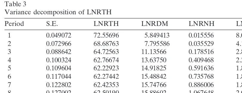
Table 3

Variance decomposition of LNRTH

Period S.E. LNRTH LNRDM LNRNH LNRJP LNRSP

1 0.049072 72.55696 5.849413 0.015556 8.017193 13.56088

2 0.072966 68.68763 7.795586 0.035529 4.185243 19.29601

3 0.088642 64.72563 11.13566 0.178516 2.836175 21.12402

4 0.100324 62.76674 13.63750 0.409468 2.215928 20.97037

5 0.109604 62.22923 14.91825 0.591636 1.887996 20.37289

6 0.117044 62.27442 15.48842 0.735768 1.801865 19.69953

7 0.122802 62.42353 15.74766 0.886006 1.893418 19.04938

8 0.127002 62.50190 15.88602 1.067648 2.087091 18.45734

9 0.129869 62.46687 15.96381 1.289950 2.331089 17.94828

10 0.131696 62.31972 15.99237 1.550755 2.592909 17.54424

11 0.132793 62.07503 15.97372 1.841025 2.848660 17.26156

12 0.133449 61.75392 15.91387 2.147436 3.078235 17.10654

Ordering: LNRDM LNRNH LNRJP LNRSP LNRTH

Notes: (1) The column S.E. is the forecast error of the variable for each forecast horizon. (2) LNRTH is the log level of Thai baht, LNRDM is the log level of Deutsche Mark, LNRNH is the log level of Dutch Guilder, LNRJP is the log level of Japanese yen, and LNRSP is the log level of Singapore dollar.

major trading partners, the Thai baht was most sensitive to the change in the Singapore dollar (except the fluctuation in the Thai baht itself). It may be because of the geographical location and similar export products of these two countries. Even when the forecast horizon was extended through 12 quarters, among Thai’s trading partners, the Singapore dollar still explained largest portion of the variance in the Thai baht. However, when the forecast horizon was increased, the Thai baht was more and more sensitive to the change in the Deutsche Mark. It shows the gradually increased linkage between the European market and the Asian market. These results also explain why the Asian currency crisis had a domino effect on worldwide financial and currency markets.

5.2. Cointegration

5.2.1. Implications of cointegration

Let X(t) be a two-dimensional difference stationary process [i.e., I(1) process].

X(t) 2 X(t21) 5 m 1 v(t) for t $1 wherem, the drift term, is a two-dimensional

vector of nonzero real numbers; andv(t), the error term, is stationary with mean zero; and each component of has a positive long-run variance. This assumption rules out deterministic trends of orders higher than or equal to quadratic. The initial value of Xi(0), i51,2, is an arbitrary random variable. Then, as shown in Eq. (24),

Xi(t) 5 mit1 X0i(t), (24)

where X0

i(t) 5 Xi(0) 1

o

t

t51vi(t). Since X0i(t) 2 X0i(t 2 1) 5 vi(t), X0i(t) is an I(1)

(19)

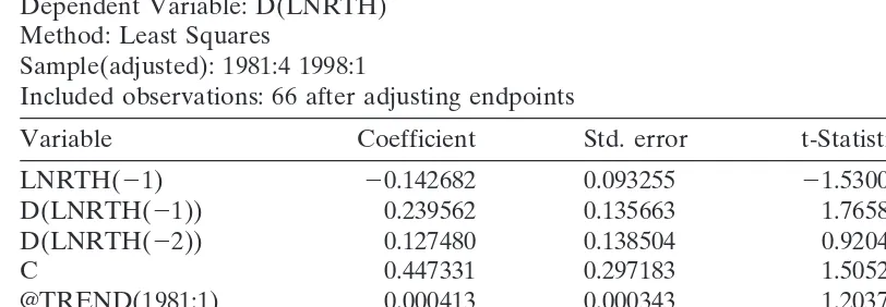
Table 4

ADF test for the log level of the Thai baht

ADF Test Statistic 21.530030 1% Critical Value* 24.1013 5% Critical Value 23.4779 10% Critical Value 23.1663 Augmented Dickey-Fuller Test Equation

Dependent Variable: D(LNRTH) Method: Least Squares

Sample(adjusted): 1981:4 1998:1

Included observations: 66 after adjusting endpoints

Variable Coefficient Std. error t-Statistic Prob.

LNRTH(21) 20.142682 0.093255 21.530030 0.1312

D(LNRTH(21)) 0.239562 0.135663 1.765858 0.0824

D(LNRTH(22)) 0.127480 0.138504 0.920403 0.3610

C 0.447331 0.297183 1.505239 0.1374

@TREND(1981:1) 0.000413 0.000343 1.203747 0.2333

R-squared 0.082624 Mean dependent var 0.007873

Adjusted R-squared 0.022469 S.D. dependent var 0.053378

S.E. of regression 0.052775 Akaike info criterion 22.972811

Sum squared resid 0.169900 Schwarz criterion 22.806928

Log likelihood 103.1028 F-statistic 1.373507

Durbin-Watson stat 1.983141 Prob(F-statistic) 0.253651

* MacKinnon critical values for rejection of hypothesis of a unit root.

Suppose thatX1(t) andX2(t) are cointegrated with a cointegrating vector (1,2b)9,

the linear combination ofX1(t)2 bX2(t) should be stationary. Eq. (24) implies Eq. (25):

X1(t) 2 bX2(t) 5(m12 bm2)t1[X01(t) 2 bX02(t)]. (25)

Therefore, the stationarity ofX1(t) 2 bX2(t) requires not only that is stationary, but

alsom12 bm250. The first requirement is calledstochasticcointegration and requires

only the stochastic components of both series to be cointegrated. It is possible that X1(t) and X2(t) are stochastically cointegrated while m12 bm2is not zero, therefore

X1(t) 2 bX2(t) is not stationary. The second requirement is called the deterministic

cointegration restriction, which implies that (1,2 b)9not only eliminates the stochastic trend but also the deterministic trend. The deterministic cointegration restriction has not been tested in most of applied economics papers using the concept of cointegration.

5.2.2. Canonical cointegrating regression (CCR)

(20)

Table 5

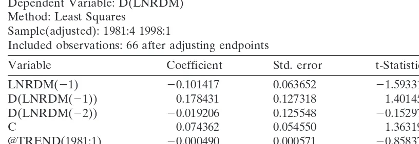
ADF test for the log level of DM

Dependent Variable: D(LNRDM) Method: Least Squares

LNRDM(21) 20.101417 0.063652 21.593317 0.1163

D(LNRDM(21)) 0.178431 0.127318 1.401459 0.1661

D(LNRDM(22)) 20.019206 0.125548 20.152977 0.8789

C 0.074362 0.054550 1.363199 0.1778

@TREND(1981:1) 20.000490 0.000571 20.858370 0.3940

asymptotic chi-square tests for the null hypothesis of cointegration which are free from nuisance parameters.

Suppose that X1(t) are cointegrated with a cointegrating vector (1,2b)9 and the

error term in the cointegrated system isε(t). Assume thatε(t) is stationary and ergodic with zero mean. Let C(i) 5 E[ε(t)ε(t 2 i)9] be the covariance function of ε(t). The long-run variance of ε(t), V, is then equal to o∞

2∞C(i). Decompose V as V 5 o 1

L 1 L9, where o 5 C(0) and L 5 o∞i51C(i). Define G 5 o 1 L, and denote each

element of V and G by corresponding lower case with subscript e.g., V 5

3

v11v12

v21v22

4

.

Then defineG25[g12,g22]9and letoˆ ,Gˆ2,bˆ ,vˆ12,vˆ22denote consistent estimators ofo,G2,

b,v12, v22. The data transformation process in the CCR is as shown in Eq. (26):

X*1(t)5 X1(t) 2

3

o

ˆ21Gˆ2bˆ 1 (0,vˆ12vˆ2221)9

4

9ε(t),

X*2(t)5 X2(t) 2

3

o

ˆ21Gˆ2

4

9ε(t). (26)

The CCR estimator is obtained by the ordinary least squares regression ofX*1(t) on

X*2(t) along with appropriate deterministic terms, as shown in Eq. (27):

X*1(t)5 uc1

o

qi51gtti1 bX*2(t) 1ε*c(t). (27)

(21)

Table 6

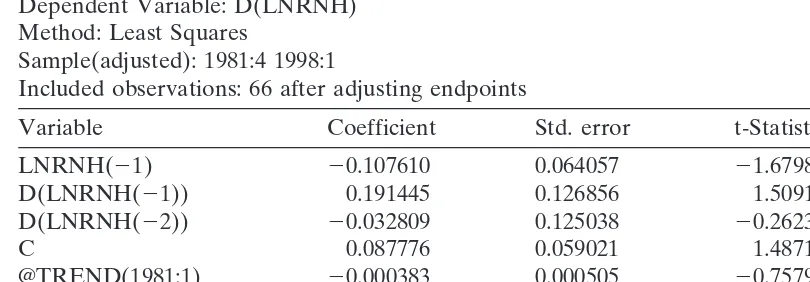
ADF test for the log level of Dutch Guilder

ADF Test Statistic 21.679896 1% Critical Value* 24.1013 5% Critical Value 23.4779

LNRNH(21) 20.107610 0.064057 21.679896 0.0981

D(LNRNH(21)) 0.191445 0.126856 1.509156 0.1364

D(LNRNH(22)) 20.032809 0.125038 20.262395 0.7939

C 0.087776 0.059021 1.487196 0.1421

@TREND(1981:1) 20.000383 0.000505 20.757954 0.4514

parameters that are required for the data transformation [Eq. (26)]. LetH(p,q)denote the standard Wald statistic to test the hypothesisgp115 gp125...5 gq50, with the

estimate of variance ofε(t) replaced by the long-run variance of the CCR. TheH(p,q) test is chi-square distributed and is free from nuisance parameters. H(0,q) tests the deterministic cointegration restriction, and H(1,q) tests the stochastic cointegration restriction. Han (1996) used Monte Carlo simulations to examine the small sample properties of the CCR test. It is found that the CCR tests performed reasonably well in terms of size and power when sample size was small.

5.2.3 Johansen VAR-based Cointegration Test

Given a group of nonstationary variables, the methodology developed by Johansen (1991, 1995) is to test the stochastic and deterministic restrictions imposed by cointegra-tion jointly. Rewriting the VAR of orderp (equation (23)) as Eq. (28),

Dyt5

P

yt211

o

Aj. Granger’s representation theorem asserts that

if the coefficient matrixPhas reduced rank r,k, then there existk 3r matricesa

and beach with rank r such that P 5 ab9 and b9ytis stationary.r is the number of

(22)

cointegrat-Table 7

ADF test for the log level of Japanese yen

Dependent Variable: D(LNRJP) Method: Least Squares

LNRJP(21) 20.066770 0.059245 21.127013 0.2642

D(LNRJP(21)) 0.161082 0.130110 1.238047 0.2204

D(LNRJP(22)) 20.012653 0.129634 20.097602 0.9226

C 0.338646 0.316453 1.070133 0.2888

@TREND(1981:1) 20.000297 0.000730 20.406394 0.6859

ing vector. The elements ofaare known as the adjustment parameters in the vector error correction model. Johansen’s method is to estimate the P matrix in an un-restricted form, then test whether one can reject the restriction implied by the reduced rank ofP. As it is mentioned above, the Johansen’s test is a joint test for the determinis-tic and stochasdeterminis-tic cointegration restrictions. Therefore, one cannot separately test each of these restrictions. When there is no cointegrating relation accepted, it may be because of either the deterministic or the stochastic restriction is violated.

5.2.4. Empirical results on tests for cointegration

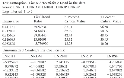
The augmented Dickey-Fuller (ADF) test is applied to perform a unit root test for the log levels of all five real exchange rates. Results are tabulated in Tables 4–8. It is found that all five series are nonstationary and I(1) process. The results provide the basis for testing cointegration. Table 9 summarizes Johansen’s LR test for cointegration between the log levels of these five real exchange rates. The LR test indicates that there is one cointegrating vector. These five real exchange rates do have a long-run relationship as a currency basket peg implies.

(23)

Table 8

ADF test for the log level of Singapore dollar

Dependent Variable: D(LNRSP) Method: Least Squares

LNRSP(21) 20.062623 0.039294 21.593692 0.1162

D(LNRSP(21)) 0.309653 0.125591 2.465572 0.0165

D(LNRSP(22)) 20.084275 0.135542 20.621768 0.5364

C 0.042511 0.027081 1.569758 0.1216

@TREND(1981:1) 20.000231 0.000203 21.135057 0.2608

exchange rates. When there is a 1 percent change against the U.S. dollar in the Deutsche Mark, the Japanese yen, the Dutch Guilder, and the Singapore dollar, the percentage change of the Thai baht against the U.S. dollar is less than 1 percent. The Thai baht was relatively inflexible, or it pegged too much to the U.S. dollar, compared to other currencies chosen in its currency basket. It also implies that the currency basket weights chosen by the Thai government may not be adequate to maintain the competitiveness of the Thai products.

(24)

Table 9

Johansen cointegration test results Sample: 1981:1 1998:1

Included observations: 66

Test assumption: Linear deterministic trend in the data Series: LNRTH LNRDM LNRNH LNRJP LNRSP Lags interval: 1 to 2

Likelihood 5 Percent 1 Percent Hypothesized

Eigenvalue Ratio Critical Value Critical Value no. of CE(s)

0.411181 89.59234 87.31 96.58 None*

0.312001 54.63630 62.99 70.05 At most 1

0.215675 29.95446 42.44 48.45 At most 2

0.116085 13.92093 25.32 30.45 At most 3

0.083808 5.776920 12.25 16.26 At most 4

Unnormalized Cointegrating Coefficients:

LNRTH LNRDM LNRNH LNRJP LNRSP @TREND(81:2)

25.325281 23.078102 2.941115 20.123515 4.205830 0.012573

0.970892 214.64932 13.63602 0.107845 0.641780 20.023955

21.033552 23.069582 2.216782 1.394651 2.647082 0.014957

0.825143 21.698328 0.046429 1.062682 21.038261 20.007093

20.433470 210.92547 11.20770 0.332703 0.033636 20.010117

Normalized Cointegrating Coefficients: 1 Cointegrating Equation(s)

LNRTH LNRDM LNRNH LNRJP LNRSP @TREND(81:2) C

1.000000 0.578017 20.552293 0.023194 20.789786 20.002361 22.750862 (0.52273) (0.49799) (0.05091) (0.06558) (0.00078)

Log likelihood 766.4269

* (**) denotes rejection of the hypothesis at 5%(1%) significance level. L.R. test indicates 1 cointegrating equation(s) at 5% significance level.

the currency basket weights for the Thai baht were not optimal and would result in the relative inflexibility of the Thai baht compared to the currencies chosen in its currency basket.

6. Conclusions

(25)

Table 10 CCR test results

Regressand: Estimated

Log Thai baht Coefficientsa _H(0,1)b _H(1,2)c _H(1,4)c _H(1,5)c

Log DM 2.098 (0.419)

Log Guilder 22.127 (0.385)

Log yen 0.046 (0.065) 0.09 0.215 0.208 0.313

Log Singapore dollar 20.864 (0.088)

Notes: Andrews and Monahan’s (1992) VAR prewhitening method together with the Andrews’ (1991) automatic bandwidth estimator are used.

a_{Standard errors are shown in parentheses.}

b_{p-values are shown in parentheses. This statistic tests the deterministic cointegration restriction.} c_{p-values are shown in parentheses. This statistic tests the stochastic cointegration restriction.}

This paper further investigates the long-run relationship between the real exchange rates in a currency basket. Using the data of Thailand and its major trading partners, the VAR results show that, between the period of 1981 Q1 and 1998 Q1, the Thai baht against the U.S. dollar depreciated following the depreciation of the Deutsche Mark and the Singapore dollar. But the comparable depreciation disappeared in about two to three quarters. By contrast, the Thai baht against the U.S. dollar first appreciated when the Japanese yen against the U.S. dollar depreciated, and then the Thai baht started to depreciate after four quarters. This unusual behavior of the Thai baht hurt the relative competitiveness of Thai products in the export market at crucial moments and led to its trade deficit. The combination of exchange rate behavior and huge current account deficits may draw the international speculators’ attention and their attacks on the Thai baht.

Based upon results from the canonical cointegrating regression and the Johansen’s LR test, the real exchange rate of the Thai baht against the U.S. dollar and its five largest trading partners are cointegrated in the long run. The estimated cointegrating vector reveals that the value of the Thai baht against the U.S. dollar was relatively stable compared to the currency values of its trading partners in the 1980–1998 period. The overall inflexibility of the Thai baht led to its overvaluation when other currencies depreciated in the past two decades. It initially cut inflationary expectation in Thailand and helped the Thai economy to grow rapidly, but it eventually resulted in a huge trade deficit, current account deficit, and the 1997 currency crisis.

Acknowledgments

(26)

Mathematical appendix

Solutions for simultaneous equations (4), (8) and (9) forpˆ0, pˆx,pˆmare

pˆ05E1(rˆ 1qˆN 2pˆ0) 1oE2i(Jˆi1qˆi2 qˆN) 1E3Gˆ

pˆx5 P1(rˆ 1qˆN 2pˆ0) 1 oP2i(Jˆi1qˆi2 qˆN) 1 P3Gˆ

pˆm5 L1(rˆ 1qˆN 2pˆ0) 1 oL2i(Jˆi1qˆi 2qˆN) 1 L3Gˆ

DefineV15ε9m2 d9m/φand V25ε90 2 d90/φ. Let D151 2k02ε90(12 u), D251 2

ε9m(1 2 u), and D351 2k9 1 V1A 2ε9mu.

E15

D1(kV1B1k9) 1D2(k0k 1kV2B)

2D1(V111 2ε9mu) 1D2(12k01ε90u 2 V2)

E2i5

D1(V1Bkai1k9bi) 1D2(k01 V2B)kai 2D1(V111 2εmu9 ) 1D2(12k01ε90u 2 V2)

E35

g9mD11 g90D2

2D1(V111 2ε9mu) 1D2(12k01ε90u 2 V2)

P15

D1(k9 2k 2kV1A 1kεmu9 ) 1D2k(1 2 V2A1 ε90u)

D1[(12k)(εm9u 2 V1) 21] 1D2[11(ε90u 2 V2)(12k)2 k(12k0)]

P2i5

D1[k9bi2 kk9bi2 (12k9 1 VA2ε9mu)kai]1 D2(12 V2A1ε90u)kai

D1[(12k)(εmu 2 V9 1) 21] 1D2[11(ε90u 2 V2)(12k) 2k(12k0)]

P35

(1 2k)(g9mD11 g90D2)

D1[(1 2k)(ε9mu 2 V1)2 1]1 D2[11 (ε90u 2 V2)(12k)2k(12k0)]

L15

(k01 V2B)[kD32 k9(12k)]1 (12 V2A1ε90u)(k9 1kV1B)

D1(2V11 kV1B2 11 k9 1ε9mu)(k01 V2B)[(12k)D22kD31k9(1 2k)]

1(12 V2A1ε90u)(D22 kV1B2 k9)

L2i 5

(k01 V2B)[D3k9ai 2(12k)k9bi]1(1 2 V2A1 ε90u)(k9bi2 V1Bkai) D1(2V11 kV1B2 11 k9 1ε9mu)(k01 V2B)[(12k)D22kD31k9(1 2k)]

1(12 V2A1ε90u)(D22 kV1B2 k9)

L35

[V1B(12k)1 D3]g01 [12 V2A1ε90u 2(1 2k)(k01 V2B)]gm D1(2V11 kV1B2 11k9 1ε9mu)(k01 V2B)[(12k)D22kD31k9(12 k)]

1 (12 V2A1ε90u)(D22kV1B2k9)

Note

(27)

currency (the U.S. dollar) at an existing official intervention rate, thus implicitly supporting commercial banks’ transactions by assuming the role of market maker. These intervention rates are liable to change in the following day for the following reasons: (1) fluctuations in the market quotations of the currencies included in the index; and (2) conditions in the domestic foreign exchange market (especially strong imbalances between supply and demand).

References

Akrasanee, N., Jansen, K., & Pongpisanupichit, J. (1991). International capital flows and economic adjustment in Thailand,Thailand Development Research Institute, Bangkok.

Andrews, D. W. K. (1991). Heteroskedasticity and autocorrelation consistent covariance matrix estima-tion.Econometrica 59, 817–858.

Andrews, D. W. K., & Monahan, C. J. (1992). An improved heteroskedasticity and autocorrelation consistent covariance matrix estimator.Econometrica 60, 953–966.

Asian Development Bank (1992). Financial Sector Policy,Asian Development Outlook, Manila. Bayoumi, T. (1994). A Formal Model of Optimum Currency Areas. International Monetary FundStaff

Papers 41, 537–54.

Branson, W. H. & Katseli, L. (1981). Currency baskets and real effective exchange rates.NBER Working Paper No. 666, April.

Chang, R., & Velasco, A. (1997). Financial Fragility and the Exchange Rate Regime. Federal Reserve Bank of Atlanta,Working Paper 97, 6.

Edison, H. J., & Melvin, M. (1990). The determinants and implications of the choice of an exchange rate system. In Haraf & Willett (Eds.),Monetary Policy for a Volatile Global Economy(pp. 1–44). AEI Press.

Engle, R. F., & Granger, C. W. J. (1987). Cointegration and error correction: Representation, estimation, and testing.Econometrica 55, 251–276.

Friedman, M. (1953). The case for flexible exchange rates. In Friedman,Essays in Positive Economics

(pp. 157–203). University of Chicago Press.

Gan, W.-B. (1994). Characterizing real exchange rate behaviour of selected East Asian economies.

Journal of Economic Development 19(2), 67–92.

Han, H.-L. (1996). Small sample properties of canonical cointegrating regressions.Empirical Economics 21, 235–253.

Hataiseree, R. (1995). Cointegration tests of purchasing power parity: The case of the Thai baht.Asian Economic Journal 9(1), 57–69.

Johansen, S. (1991). Estimation and Hypothesis Testing of Cointegration Vectors in Gaussian Vector Autoregressive Models.Econometrica 59, 1551–1580.

Johansen, S. (1995).Likelihood-based Inference in Cointegrated Vector Autoregressive Models.Oxford University Press.

Kenen, P. (1969). The theory of optimum currency areas: An eclective view. In Mundell & Swoboda (Eds.), pp. 41–60.

Krugman, P. (1991). Target zones and exchange rate dynamics.Quarterly Journal of Economics 106, 669–82.

Mackinnon, J. G. (1991). Critical values for cointegration tests. In R. F. engle & C. W. J. Granger (Eds.),

Long-run Economic Relationships: Readings in Cointegration, Oxford University Press. McKinnon, R. I. (1963). Optimal currency area.American Economic Review 53, 717–25.

Mundell, R. A. (1969). Problems of the international monetary system. In Mundell and Swoboda (Eds.), pp. 21–38.

(28)

Phillips, P. C. B., & Ouliaris, S. (1988). Testing for cointegration using principal components methods.

Journal of Economic Dynamics and Control,, 205–230.

Robinson, D., Byeon, Y., Teja, R., & Tseng, W. (1991). Thailand: Adjust to success current policy issues.

Occasional Paper No. 85.Washington, D.C.: International Monetary Fund.

Wibulswasdi, C. (1987). Thai experience in economic management during 1980–87.Bank of Thailand Quarterly Bulletin 27, 31–46.