Spark: The Definitive Guide
Big Data Processing Made Simple
Spark: The Definitive Guide
by Bill Chambers and Matei Zaharia
Copyright © 2018 Databricks. All rights reserved. Printed in the United States of America.
Published by O’Reilly Media, Inc., 1005 Gravenstein Highway North, Sebastopol, CA 95472. O’Reilly books may be purchased for educational, business, or sales promotional use. Online
editions are also available for most titles (http://oreilly.com/safari). For more information, contact our corporate/institutional sales department: 800-998-9938 or [email protected].
Editor: Nicole Tache
Production Editor: Justin Billing
Copyeditor: Octal Publishing, Inc., Chris Edwards, and Amanda Kersey
Proofreader: Jasmine Kwityn
Indexer: Judith McConville
Interior Designer: David Futato
Cover Designer: Karen Montgomery
Illustrator: Rebecca Demarest
February 2018: First Edition
Revision History for the First Edition
2018-02-08: First Release
See http://oreilly.com/catalog/errata.csp?isbn=9781491912218 for release details.
The O’Reilly logo is a registered trademark of O’Reilly Media, Inc. Spark: The Definitive Guide, the cover image, and related trade dress are trademarks of O’Reilly Media, Inc. Apache, Spark and Apache Spark are trademarks of the Apache Software Foundation.
While the publisher and the authors have used good faith efforts to ensure that the information and instructions contained in this work are accurate, the publisher and the authors disclaim all
responsibility for errors or omissions, including without limitation responsibility for damages
this work is at your own risk. If any code samples or other technology this work contains or describes is subject to open source licenses or the intellectual property rights of others, it is your responsibility to ensure that your use thereof complies with such licenses and/or rights.
Preface
Welcome to this first edition of Spark: The Definitive Guide! We are excited to bring you the most complete resource on Apache Spark today, focusing especially on the new generation of Spark APIs introduced in Spark 2.0.
Apache Spark is currently one of the most popular systems for large-scale data processing, with APIs in multiple programming languages and a wealth of built-in and third-party libraries. Although the project has existed for multiple years—first as a research project started at UC Berkeley in 2009, then at the Apache Software Foundation since 2013—the open source community is continuing to build more powerful APIs and high-level libraries over Spark, so there is still a lot to write about the project. We decided to write this book for two reasons. First, we wanted to present the most
comprehensive book on Apache Spark, covering all of the fundamental use cases with easy-to-run examples. Second, we especially wanted to explore the higher-level “structured” APIs that were finalized in Apache Spark 2.0—namely DataFrames, Datasets, Spark SQL, and Structured Streaming —which older books on Spark don’t always include. We hope this book gives you a solid foundation to write modern Apache Spark applications using all the available tools in the project.
In this preface, we’ll tell you a little bit about our background, and explain who this book is for and how we have organized the material. We also want to thank the numerous people who helped edit and review this book, without whom it would not have been possible.
About the Authors
Both of the book’s authors have been involved in Apache Spark for a long time, so we are very excited to be able to bring you this book.
Bill Chambers started using Spark in 2014 on several research projects. Currently, Bill is a Product Manager at Databricks where he focuses on enabling users to write various types of Apache Spark applications. Bill also regularly blogs about Spark and presents at conferences and meetups on the topic. Bill holds a Master’s in Information Management and Systems from the UC Berkeley School of Information.
Matei Zaharia started the Spark project in 2009, during his time as a PhD student at UC Berkeley. Matei worked with other Berkeley researchers and external collaborators to design the core Spark APIs and grow the Spark community, and has continued to be involved in new initiatives such as the structured APIs and Structured Streaming. In 2013, Matei and other members of the Berkeley Spark team co-founded Databricks to further grow the open source project and provide commercial
Who This Book Is For
We designed this book mainly for data scientists and data engineers looking to use Apache Spark. The two roles have slightly different needs, but in reality, most application development covers a bit of both, so we think the material will be useful in both cases. Specifically, in our minds, the data scientist workload focuses more on interactively querying data to answer questions and build
statistical models, while the data engineer job focuses on writing maintainable, repeatable production applications—either to use the data scientist’s models in practice, or just to prepare data for further analysis (e.g., building a data ingest pipeline). However, we often see with Spark that these roles blur. For instance, data scientists are able to package production applications without too much hassle and data engineers use interactive analysis to understand and inspect their data to build and maintain pipelines.
While we tried to provide everything data scientists and engineers need to get started, there are some things we didn’t have space to focus on in this book. First, this book does not include in-depth
introductions to some of the analytics techniques you can use in Apache Spark, such as machine
learning. Instead, we show you how to invoke these techniques using libraries in Spark, assuming you already have a basic background in machine learning. Many full, standalone books exist to cover these techniques in formal detail, so we recommend starting with those if you want to learn about these areas. Second, this book focuses more on application development than on operations and administration (e.g., how to manage an Apache Spark cluster with dozens of users). Nonetheless, we have tried to include comprehensive material on monitoring, debugging, and configuration in Parts V
and VI of the book to help engineers get their application running efficiently and tackle day-to-day maintenance. Finally, this book places less emphasis on the older, lower-level APIs in Spark— specifically RDDs and DStreams—to introduce most of the concepts using the newer, higher-level structured APIs. Thus, the book may not be the best fit if you need to maintain an old RDD or DStream application, but should be a great introduction to writing new applications.
Conventions Used in This Book
The following typographical conventions are used in this book:
Italic
Indicates new terms, URLs, email addresses, filenames, and file extensions. Constant width
Used for program listings, as well as within paragraphs to refer to program elements such as variable or function names, databases, data types, environment variables, statements, and keywords.
Constant width bold
Constant width italic
Shows text that should be replaced with user-supplied values or by values determined by context.
TIP
This element signifies a tip or suggestion.
NOTE
This element signifies a general note.
WARNING
This element indicates a warning or caution.
Using Code Examples
We’re very excited to have designed this book so that all of the code content is runnable on real data. We wrote the whole book using Databricks notebooks and have posted the data and related material on GitHub. This means that you can run and edit all the code as you follow along, or copy it into working code in your own applications.
We tried to use real data wherever possible to illustrate the challenges you’ll run into while building large-scale data applications. Finally, we also include several larger standalone applications in the book’s GitHub repository for examples that it does not make sense to show inline in the text.
The GitHub repository will remain a living document as we update based on Spark’s progress. Be sure to follow updates there.
This book is here to help you get your job done. In general, if example code is offered with this book, you may use it in your programs and documentation. You do not need to contact us for permission unless you’re reproducing a significant portion of the code. For example, writing a program that uses several chunks of code from this book does not require permission. Selling or distributing a CD-ROM of examples from O’Reilly books does require permission. Answering a question by citing this book and quoting example code does not require permission. Incorporating a significant amount of example code from this book into your product’s documentation does require permission.
We appreciate, but do not require, attribution. An attribution usually includes the title, author, publisher, and ISBN. For example: “Spark: The Definitive Guide by Bill Chambers and Matei Zaharia (O’Reilly). Copyright 2018 Databricks, Inc., 978-1-491-91221-8.”
contact us at [email protected].
O’Reilly Safari
Safari (formerly Safari Books Online) is a membership-based training and reference platform for enterprise, government, educators, and individuals.
Members have access to thousands of books, training videos, Learning Paths, interactive tutorials, and curated playlists from over 250 publishers, including O’Reilly Media, Harvard Business Review, Prentice Hall Professional, Addison-Wesley Professional, Microsoft Press, Sams, Que, Peachpit Press, Adobe, Focal Press, Cisco Press, John Wiley & Sons, Syngress, Morgan Kaufmann, IBM Redbooks, Packt, Adobe Press, FT Press, Apress, Manning, New Riders, McGraw-Hill, Jones & Bartlett, and Course Technology, among others.
For more information, please visit http://oreilly.com/safari.
How to Contact Us
Please address comments and questions concerning this book to the publisher:
O’Reilly Media, Inc.
1005 Gravenstein Highway North
Sebastopol, CA 95472
800-998-9938 (in the United States or Canada)
707-829-0515 (international or local)
707-829-0104 (fax)
To comment or ask technical questions about this book, send email to [email protected]. For more information about our books, courses, conferences, and news, see our website at
http://www.oreilly.com.
Find us on Facebook: http://facebook.com/oreilly
Follow us on Twitter: http://twitter.com/oreillymedia
Watch us on YouTube: http://www.youtube.com/oreillymedia
There were a huge number of people that made this book possible.
First, we would like to thank our employer, Databricks, for allocating time for us to work on this book. Without the support of the company, this book would not have been possible. In particular, we would like to thank Ali Ghodsi, Ion Stoica, and Patrick Wendell for their support.
Additionally, there are numerous people that read drafts of the book and individual chapters. Our reviewers were best-in-class, and provided invaluable feedback.
These reviewers, in alphabetical order by last name, are: Lynn Armstrong
Mikio Braun Jules Damji Denny Lee Alex Thomas
In addition to the formal book reviewers, there were numerous other Spark users, contributors, and committers who read over specific chapters or helped formulate how topics should be discussed. In alphabetical order by last name, the people who helped are:
Josh Rosen Srinath Shankar Takuya Ueshin Herman van Hövell Reynold Xin
Philip Yang Burak Yavuz Shixiong Zhu
Chapter 1. What Is Apache Spark?
Apache Spark is a unified computing engine and a set of libraries for parallel data processing on computer clusters. As of this writing, Spark is the most actively developed open source engine for this task, making it a standard tool for any developer or data scientist interested in big data. Spark supports multiple widely used programming languages (Python, Java, Scala, and R), includes
libraries for diverse tasks ranging from SQL to streaming and machine learning, and runs anywhere from a laptop to a cluster of thousands of servers. This makes it an easy system to start with and scale-up to big data processing or incredibly large scale.
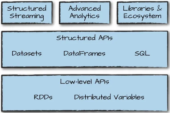
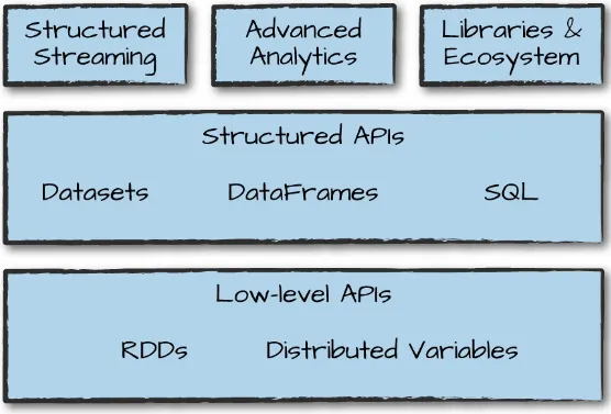
Figure 1-1 illustrates all the components and libraries Spark offers to end-users.
Figure 1-1. Spark’s toolkit
You’ll notice the categories roughly correspond to the different parts of this book. That should really come as no surprise; our goal here is to educate you on all aspects of Spark, and Spark is composed of a number of different components.
Spark as well as the context it was developed in (why is everyone suddenly excited about parallel data processing?) and its history. We will also outline the first few steps to running Spark.
Apache Spark’s Philosophy
Let’s break down our description of Apache Spark—a unified computing engine and set of libraries for big data—into its key components:
Unified
Spark’s key driving goal is to offer a unified platform for writing big data applications. What do we mean by unified? Spark is designed to support a wide range of data analytics tasks, ranging from simple data loading and SQL queries to machine learning and streaming computation, over the same computing engine and with a consistent set of APIs. The main insight behind this goal is that real-world data analytics tasks—whether they are interactive analytics in a tool such as a Jupyter notebook, or traditional software development for production applications—tend to combine many different processing types and libraries.
Spark’s unified nature makes these tasks both easier and more efficient to write. First, Spark provides consistent, composable APIs that you can use to build an application out of smaller pieces or out of existing libraries. It also makes it easy for you to write your own analytics libraries on top. However, composable APIs are not enough: Spark’s APIs are also designed to enable high performance by optimizing across the different libraries and functions composed together in a user program. For example, if you load data using a SQL query and then evaluate a machine learning model over it using Spark’s ML library, the engine can combine these steps into one scan over the data. The combination of general APIs and high-performance execution, no matter how you combine them, makes Spark a powerful platform for interactive and production applications.
Spark’s focus on defining a unified platform is the same idea behind unified platforms in other areas of software. For example, data scientists benefit from a unified set of libraries (e.g., Python or R) when doing modeling, and web developers benefit from unified frameworks such as
Node.js or Django. Before Spark, no open source systems tried to provide this type of unified engine for parallel data processing, meaning that users had to stitch together an application out of multiple APIs and systems. Thus, Spark quickly became the standard for this type of development. Over time, Spark has continued to expand its built-in APIs to cover more workloads. At the same time, the project’s developers have continued to refine its theme of a unified engine. In particular, one major focus of this book will be the “structured APIs” (DataFrames, Datasets, and SQL) that were finalized in Spark 2.0 to enable more powerful optimization under user applications.
Computing engine
of persistent storage systems, including cloud storage systems such as Azure Storage and Amazon S3, distributed file systems such as Apache Hadoop, key-value stores such as Apache Cassandra, and message buses such as Apache Kafka. However, Spark neither stores data long term itself, nor favors one over another. The key motivation here is that most data already resides in a mix of storage systems. Data is expensive to move so Spark focuses on performing computations over the data, no matter where it resides. In user-facing APIs, Spark works hard to make these storage systems look largely similar so that applications do not need to worry about where their data is. Spark’s focus on computation makes it different from earlier big data software platforms such as Apache Hadoop. Hadoop included both a storage system (the Hadoop file system, designed for low-cost storage over clusters of commodity servers) and a computing system (MapReduce), which were closely integrated together. However, this choice makes it difficult to run one of the systems without the other. More important, this choice also makes it a challenge to write
applications that access data stored anywhere else. Although Spark runs well on Hadoop storage, today it is also used broadly in environments for which the Hadoop architecture does not make sense, such as the public cloud (where storage can be purchased separately from computing) or streaming applications.
Libraries
Spark’s final component is its libraries, which build on its design as a unified engine to provide a unified API for common data analysis tasks. Spark supports both standard libraries that ship with the engine as well as a wide array of external libraries published as third-party packages by the open source communities. Today, Spark’s standard libraries are actually the bulk of the open source project: the Spark core engine itself has changed little since it was first released, but the libraries have grown to provide more and more types of functionality. Spark includes libraries for SQL and structured data (Spark SQL), machine learning (MLlib), stream processing (Spark
Streaming and the newer Structured Streaming), and graph analytics (GraphX). Beyond these libraries, there are hundreds of open source external libraries ranging from connectors for various storage systems to machine learning algorithms. One index of external libraries is available at
spark-packages.org.
Context: The Big Data Problem
Why do we need a new engine and programming model for data analytics in the first place? As with many trends in computing, this is due to changes in the economic factors that underlie computer applications and hardware.
improved processor speeds to scale up to larger computations and larger volumes of data over time. Unfortunately, this trend in hardware stopped around 2005: due to hard limits in heat dissipation, hardware developers stopped making individual processors faster, and switched toward adding more parallel CPU cores all running at the same speed. This change meant that suddenly applications
needed to be modified to add parallelism in order to run faster, which set the stage for new programming models such as Apache Spark.
On top of that, the technologies for storing and collecting data did not slow down appreciably in 2005, when processor speeds did. The cost to store 1 TB of data continues to drop by roughly two times every 14 months, meaning that it is very inexpensive for organizations of all sizes to store large amounts of data. Moreover, many of the technologies for collecting data (sensors, cameras, public datasets, etc.) continue to drop in cost and improve in resolution. For example, camera technology continues to improve in resolution and drop in cost per pixel every year, to the point where a 12-megapixel webcam costs only $3 to $4; this has made it inexpensive to collect a wide range of visual data, whether from people filming video or automated sensors in an industrial setting. Moreover, cameras are themselves the key sensors in other data collection devices, such as telescopes and even gene-sequencing machines, driving the cost of these technologies down as well.
The end result is a world in which collecting data is extremely inexpensive—many organizations today even consider it negligent not to log data of possible relevance to the business—but processing it requires large, parallel computations, often on clusters of machines. Moreover, in this new world, the software developed in the past 50 years cannot automatically scale up, and neither can the
traditional programming models for data processing applications, creating the need for new programming models. It is this world that Apache Spark was built for.
History of Spark
Apache Spark began at UC Berkeley in 2009 as the Spark research project, which was first published the following year in a paper entitled “Spark: Cluster Computing with Working Sets” by Matei
Zaharia, Mosharaf Chowdhury, Michael Franklin, Scott Shenker, and Ion Stoica of the UC Berkeley AMPlab. At the time, Hadoop MapReduce was the dominant parallel programming engine for
clusters, being the first open source system to tackle data-parallel processing on clusters of thousands of nodes. The AMPlab had worked with multiple early MapReduce users to understand the benefits and drawbacks of this new programming model, and was therefore able to synthesize a list of
problems across several use cases and begin designing more general computing platforms. In
addition, Zaharia had also worked with Hadoop users at UC Berkeley to understand their needs for the platform—specifically, teams that were doing large-scale machine learning using iterative algorithms that need to make multiple passes over the data.
Across these conversations, two things were clear. First, cluster computing held tremendous
however, the MapReduce engine made it both challenging and inefficient to build large applications. For example, the typical machine learning algorithm might need to make 10 or 20 passes over the data, and in MapReduce, each pass had to be written as a separate MapReduce job, which had to be launched separately on the cluster and load the data from scratch.
To address this problem, the Spark team first designed an API based on functional programming that could succinctly express multistep applications. The team then implemented this API over a new engine that could perform efficient, in-memory data sharing across computation steps. The team also began testing this system with both Berkeley and external users.
The first version of Spark supported only batch applications, but soon enough another compelling use case became clear: interactive data science and ad hoc queries. By simply plugging the Scala
interpreter into Spark, the project could provide a highly usable interactive system for running queries on hundreds of machines. The AMPlab also quickly built on this idea to develop Shark, an engine that could run SQL queries over Spark and enable interactive use by analysts as well as data scientists. Shark was first released in 2011.
After these initial releases, it quickly became clear that the most powerful additions to Spark would be new libraries, and so the project began to follow the “standard library” approach it has today. In particular, different AMPlab groups started MLlib, Spark Streaming, and GraphX. They also ensured that these APIs would be highly interoperable, enabling writing end-to-end big data applications in the same engine for the first time.
In 2013, the project had grown to widespread use, with more than 100 contributors from more than 30 organizations outside UC Berkeley. The AMPlab contributed Spark to the Apache Software
Foundation as a long-term, vendor-independent home for the project. The early AMPlab team also launched a company, Databricks, to harden the project, joining the community of other companies and organizations contributing to Spark. Since that time, the Apache Spark community released Spark 1.0 in 2014 and Spark 2.0 in 2016, and continues to make regular releases, bringing new features into the project.
Finally, Spark’s core idea of composable APIs has also been refined over time. Early versions of Spark (before 1.0) largely defined this API in terms of functional operations—parallel operations such as maps and reduces over collections of Java objects. Beginning with 1.0, the project added Spark SQL, a new API for working with structured data—tables with a fixed data format that is not tied to Java’s in-memory representation. Spark SQL enabled powerful new optimizations across libraries and APIs by understanding both the data format and the user code that runs on it in more detail. Over time, the project added a plethora of new APIs that build on this more powerful
structured foundation, including DataFrames, machine learning pipelines, and Structured Streaming, a high-level, automatically optimized streaming API. In this book, we will spend a signficant amount of time explaining these next-generation APIs, most of which are marked as production-ready.
Spark has been around for a number of years but continues to gain in popularity and use cases. Many new projects within the Spark ecosystem continue to push the boundaries of what’s possible with the system. For example, a new high-level streaming engine, Structured Streaming, was introduced in 2016. This technology is a huge part of companies solving massive-scale data challenges, from technology companies like Uber and Netflix using Spark’s streaming and machine learning tools, to institutions like NASA, CERN, and the Broad Institute of MIT and Harvard applying Spark to scientific data analysis.
Spark will continue to be a cornerstone of companies doing big data analysis for the foreseeable future, especially given that the project is still developing quickly. Any data scientist or engineer who needs to solve big data problems probably needs a copy of Spark on their machine—and hopefully, a copy of this book on their bookshelf!
Running Spark
This book contains an abundance of Spark-related code, and it’s essential that you’re prepared to run it as you learn. For the most part, you’ll want to run the code interactively so that you can experiment with it. Let’s go over some of your options before we begin working with the coding parts of the book.
You can use Spark from Python, Java, Scala, R, or SQL. Spark itself is written in Scala, and runs on the Java Virtual Machine (JVM), so therefore to run Spark either on your laptop or a cluster, all you need is an installation of Java. If you want to use the Python API, you will also need a Python
interpreter (version 2.7 or later). If you want to use R, you will need a version of R on your machine. There are two options we recommend for getting started with Spark: downloading and installing Apache Spark on your laptop, or running a web-based version in Databricks Community Edition, a free cloud environment for learning Spark that includes the code in this book. We explain both of those options next.
Downloading Spark Locally
If you want to download and run Spark locally, the first step is to make sure that you have Java installed on your machine (available as java), as well as a Python version if you would like to use Python. Next, visit the project’s official download page, select the package type of “Pre-built for Hadoop 2.7 and later,” and click “Direct Download.” This downloads a compressed TAR file, or tarball, that you will then need to extract. The majority of this book was written using Spark 2.2, so downloading version 2.2 or later should be a good starting point.
Downloading Spark for a Hadoop cluster
http://spark.apache.org/downloads.html by selecting a different package type. We discuss how Spark runs on clusters and the Hadoop file system in later chapters, but at this point we recommend just running Spark on your laptop to start out.
NOTE
In Spark 2.2, the developers also added the ability to install Spark for Python via pip install pyspark. This functionality came out as this book was being written, so we weren’t able to include all of the relevant instructions.
Building Spark from source
We won’t cover this in the book, but you can also build and configure Spark from source. You can select a source package on the Apache download page to get just the source and follow the
instructions in the README file for building.
After you’ve downloaded Spark, you’ll want to open a command-line prompt and extract the package. In our case, we’re installing Spark 2.2. The following is a code snippet that you can run on any Unix-style command line to unzip the file you downloaded from Spark and move into the directory:
cd~/Downloads
tar-xfspark-2.2.0-bin-hadoop2.7.tgz cdspark-2.2.0-bin-hadoop2.7.tgz
Note that Spark has a large number of directories and files within the project. Don’t be intimidated! Most of these directories are relevant only if you’re reading source code. The next section will cover the most important directories—the ones that let us launch Spark’s different consoles for interactive use.
Launching Spark’s Interactive Consoles
You can start an interactive shell in Spark for several different programming languages. The majority of this book is written with Python, Scala, and SQL in mind; thus, those are our recommended starting points.
Launching the Python console
You’ll need Python 2 or 3 installed in order to launch the Python console. From Spark’s home directory, run the following code:
./bin/pyspark
Launching the Scala console
To launch the Scala console, you will need to run the following command:
./bin/spark-shell
After you’ve done that, type “spark” and press Enter. As in Python, you’ll see the SparkSession object, which we cover in Chapter 2.
Launching the SQL console
Parts of this book will cover a large amount of Spark SQL. For those, you might want to start the SQL console. We’ll revisit some of the more relevant details after we actually cover these topics in the book.
./bin/spark-sql
Running Spark in the Cloud
If you would like to have a simple, interactive notebook experience for learning Spark, you might prefer using Databricks Community Edition. Databricks, as we mentioned earlier, is a company founded by the Berkeley team that started Spark, and offers a free community edition of its cloud service as a learning environment. The Databricks Community Edition includes a copy of all the data and code examples for this book, making it easy to quickly run any of them. To use the Databricks Community Edition, follow the instructions at https://github.com/databricks/Spark-The-Definitive-Guide. You will be able to use Scala, Python, SQL, or R from a web browser–based interface to run and visualize results.
Data Used in This Book
We’ll use a number of data sources in this book for our examples. If you want to run the code locally, you can download them from the official code repository in this book as desribed at
Chapter 2. A Gentle Introduction to Spark
Now that our history lesson on Apache Spark is completed, it’s time to begin using and applying it! This chapter presents a gentle introduction to Spark, in which we will walk through the core
architecture of a cluster, Spark Application, and Spark’s structured APIs using DataFrames and SQL. Along the way we will touch on Spark’s core terminology and concepts so that you can begin using Spark right away. Let’s get started with some basic background information.
Spark’s Basic Architecture
Typically, when you think of a “computer,” you think about one machine sitting on your desk at home or at work. This machine works perfectly well for watching movies or working with spreadsheet software. However, as many users likely experience at some point, there are some things that your computer is not powerful enough to perform. One particularly challenging area is data processing. Single machines do not have enough power and resources to perform computations on huge amounts of information (or the user probably does not have the time to wait for the computation to finish). A
cluster, or group, of computers, pools the resources of many machines together, giving us the ability
to use all the cumulative resources as if they were a single computer. Now, a group of machines alone is not powerful, you need a framework to coordinate work across them. Spark does just that,
managing and coordinating the execution of tasks on data across a cluster of computers.
The cluster of machines that Spark will use to execute tasks is managed by a cluster manager like Spark’s standalone cluster manager, YARN, or Mesos. We then submit Spark Applications to these cluster managers, which will grant resources to our application so that we can complete our work.
Spark Applications
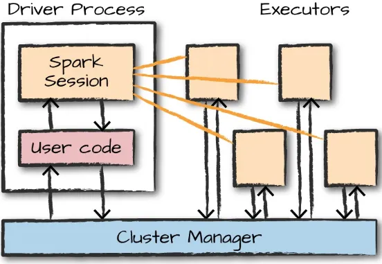
Spark Applications consist of a driver process and a set of executor processes. The driver process runs your main() function, sits on a node in the cluster, and is responsible for three things: maintaining information about the Spark Application; responding to a user’s program or input; and analyzing, distributing, and scheduling work across the executors (discussed momentarily). The driver process is absolutely essential—it’s the heart of a Spark Application and maintains all relevant information during the lifetime of the application.
The executors are responsible for actually carrying out the work that the driver assigns them. This
means that each executor is responsible for only two things: executing code assigned to it by the driver, and reporting the state of the computation on that executor back to the driver node.
cluster at the same time. We will discuss cluster managers more in Part IV.
Figure 2-1. The architecture of a Spark Application
In Figure 2-1, we can see the driver on the left and four executors on the right. In this diagram, we removed the concept of cluster nodes. The user can specify how many executors should fall on each node through configurations.
NOTE
Spark, in addition to its cluster mode, also has a local mode. The driver and executors are simply processes, which means that they can live on the same machine or different machines. In local mode, the driver and executurs run (as threads) on your individual computer instead of a cluster. We wrote this book with local mode in mind, so you should be able to run everything on a single machine.
Here are the key points to understand about Spark Applications at this point:
Spark employs a cluster manager that keeps track of the resources available.
The executors, for the most part, will always be running Spark code. However, the driver can be “driven” from a number of different languages through Spark’s language APIs. Let’s take a look at those in the next section.
Spark’s Language APIs
Spark’s language APIs make it possible for you to run Spark code using various programming
languages. For the most part, Spark presents some core “concepts” in every language; these concepts are then translated into Spark code that runs on the cluster of machines. If you use just the Structured APIs, you can expect all languages to have similar performance characteristics. Here’s a brief rundown:
Scala
Spark is primarily written in Scala, making it Spark’s “default” language. This book will include Scala code examples wherever relevant.
Java
Even though Spark is written in Scala, Spark’s authors have been careful to ensure that you can write Spark code in Java. This book will focus primarily on Scala but will provide Java
examples where relevant. Python
Python supports nearly all constructs that Scala supports. This book will include Python code examples whenever we include Scala code examples and a Python API exists.
SQL
Spark supports a subset of the ANSI SQL 2003 standard. This makes it easy for analysts and non-programmers to take advantage of the big data powers of Spark. This book includes SQL code examples wherever relevant.
R
Spark has two commonly used R libraries: one as a part of Spark core (SparkR) and another as an R community-driven package (sparklyr). We cover both of these integrations in Chapter 32.
Figure 2-2. The relationship between the SparkSession and Spark’s Language API
Each language API maintains the same core concepts that we described earlier. There is a
SparkSession object available to the user, which is the entrance point to running Spark code. When using Spark from Python or R, you don’t write explicit JVM instructions; instead, you write Python and R code that Spark translates into code that it then can run on the executor JVMs.
Spark’s APIs
Although you can drive Spark from a variety of languages, what it makes available in those languages is worth mentioning. Spark has two fundamental sets of APIs: the low-level “unstructured” APIs, and the higher-level structured APIs. We discuss both in this book, but these introductory chapters will focus primarily on the higher-level structured APIs.
Starting Spark
Thus far, we covered the basic concepts of Spark Applications. This has all been conceptual in
nature. When we actually go about writing our Spark Application, we are going to need a way to send user commands and data to it. We do that by first creating a SparkSession.
NOTE
To do this, we will start Spark’s local mode, just like we did in Chapter 1. This means running ./bin/spark-shell to access the Scala console to start an interactive session. You can also start the Python console by using ./bin/pyspark. This starts an interactive Spark Application. There is also a process for submitting standalone applications to Spark called spark-submit, whereby you can submit a precompiled application to Spark. We’ll show you how to do that in Chapter 3.
When you start Spark in this interactive mode, you implicitly create a SparkSession that manages the Spark Application. When you start it through a standalone application, you must create the
The SparkSession
As discussed in the beginning of this chapter, you control your Spark Application through a driver process called the SparkSession. The SparkSession instance is the way Spark executes user-defined manipulations across the cluster. There is a one-to-one correspondence between a SparkSession and a Spark Application. In Scala and Python, the variable is available as spark when you start the
console. Let’s go ahead and look at the SparkSession in both Scala and/or Python:
spark
In Scala, you should see something like the following:
res0: org.apache.spark.sql.SparkSession = org.apache.spark.sql.SparkSession@...
In Python you’ll see something like this:
<pyspark.sql.session.SparkSession at 0x7efda4c1ccd0>
Let’s now perform the simple task of creating a range of numbers. This range of numbers is just like a named column in a spreadsheet:
// in Scala
valmyRange=spark.range(1000).toDF("number") # in Python
myRange=spark.range(1000).toDF("number")
You just ran your first Spark code! We created a DataFrame with one column containing 1,000 rows with values from 0 to 999. This range of numbers represents a distributed collection. When run on a cluster, each part of this range of numbers exists on a different executor. This is a Spark DataFrame.
DataFrames
A DataFrame is the most common Structured API and simply represents a table of data with rows and columns. The list that defines the columns and the types within those columns is called the schema. You can think of a DataFrame as a spreadsheet with named columns. Figure 2-3 illustrates the
fundamental difference: a spreadsheet sits on one computer in one specific location, whereas a Spark DataFrame can span thousands of computers. The reason for putting the data on more than one
Figure 2-3. Distributed versus single-machine analysis
The DataFrame concept is not unique to Spark. R and Python both have similar concepts. However, Python/R DataFrames (with some exceptions) exist on one machine rather than multiple machines. This limits what you can do with a given DataFrame to the resources that exist on that specific machine. However, because Spark has language interfaces for both Python and R, it’s quite easy to convert Pandas (Python) DataFrames to Spark DataFrames, and R DataFrames to Spark DataFrames.
NOTE
Spark has several core abstractions: Datasets, DataFrames, SQL Tables, and Resilient Distributed Datasets (RDDs). These different abstractions all represent distributed collections of data. The easiest and most efficient are DataFrames, which are available in all languages. We cover Datasets at the end of Part II, and RDDs in Part III.
Partitions
To allow every executor to perform work in parallel, Spark breaks up the data into chunks called
partitions. A partition is a collection of rows that sit on one physical machine in your cluster. A
DataFrame’s partitions represent how the data is physically distributed across the cluster of machines during execution. If you have one partition, Spark will have a parallelism of only one, even if you have thousands of executors. If you have many partitions but only one executor, Spark will still have a parallelism of only one because there is only one computation resource.
An important thing to note is that with DataFrames you do not (for the most part) manipulate partitions manually or individually. You simply specify high-level transformations of data in the physical
partitions, and Spark determines how this work will actually execute on the cluster. Lower-level APIs do exist (via the RDD interface), and we cover those in Part III.
Transformations
created. This might seem like a strange concept at first: if you cannot change it, how are you supposed to use it? To “change” a DataFrame, you need to instruct Spark how you would like to modify it to do what you want. These instructions are called transformations. Let’s perform a simple transformation to find all even numbers in our current DataFrame:
// in Scala
valdivisBy2=myRange.where("number % 2 = 0") # in Python
divisBy2=myRange.where("number % 2 = 0")
Notice that these return no output. This is because we specified only an abstract transformation, and Spark will not act on transformations until we call an action (we discuss this shortly).
Transformations are the core of how you express your business logic using Spark. There are two types of transformations: those that specify narrow dependencies, and those that specify wide
dependencies.
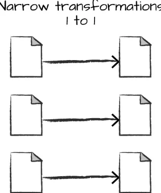
Transformations consisting of narrow dependencies (we’ll call them narrow transformations) are those for which each input partition will contribute to only one output partition. In the preceding code snippet, the where statement specifies a narrow dependency, where only one partition contributes to at most one output partition, as you can see in Figure 2-4.
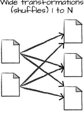
A wide dependency (or wide transformation) style transformation will have input partitions
contributing to many output partitions. You will often hear this referred to as a shuffle whereby Spark will exchange partitions across the cluster. With narrow transformations, Spark will automatically perform an operation called pipelining, meaning that if we specify multiple filters on DataFrames, they’ll all be performed in-memory. The same cannot be said for shuffles. When we perform a shuffle, Spark writes the results to disk. Wide transformations are illustrated in Figure 2-5.
Figure 2-5. A wide dependency
You’ll see a lot of discussion about shuffle optimization across the web because it’s an important topic, but for now, all you need to understand is that there are two kinds of transformations. You now can see how transformations are simply ways of specifying different series of data manipulation. This leads us to a topic called lazy evaluation.
Lazy Evaluation
Lazy evaulation means that Spark will wait until the very last moment to execute the graph of
end. An example of this is something called predicate pushdown on DataFrames. If we build a large Spark job but specify a filter at the end that only requires us to fetch one row from our source data, the most efficient way to execute this is to access the single record that we need. Spark will actually optimize this for us by pushing the filter down automatically.
Actions
Transformations allow us to build up our logical transformation plan. To trigger the computation, we run an action. An action instructs Spark to compute a result from a series of transformations. The simplest action is count, which gives us the total number of records in the DataFrame:
divisBy2.count()
The output of the preceding code should be 500. Of course, count is not the only action. There are three kinds of actions:
Actions to view data in the console
Actions to collect data to native objects in the respective language Actions to write to output data sources
In specifying this action, we started a Spark job that runs our filter transformation (a narrow transformation), then an aggregation (a wide transformation) that performs the counts on a per partition basis, and then a collect, which brings our result to a native object in the respective
language. You can see all of this by inspecting the Spark UI, a tool included in Spark with which you can monitor the Spark jobs running on a cluster.
Spark UI
Figure 2-6. The Spark UI
This chapter will not go into detail about Spark job execution and the Spark UI. We will cover that in
Chapter 18. At this point, all you need to understand is that a Spark job represents a set of
transformations triggered by an individual action, and you can monitor that job from the Spark UI.
An End-to-End Example
In the previous example, we created a DataFrame of a range of numbers; not exactly groundbreaking big data. In this section, we will reinforce everything we learned previously in this chapter with a more realistic example, and explain step by step what is happening under the hood. We’ll use Spark to analyze some flight data from the United States Bureau of Transportation statistics.
Inside of the CSV folder, you’ll see that we have a number of files. There’s also a number of other folders with different file formats, which we discuss in Chapter 9. For now, let’s focus on the CSV files.
Each file has a number of rows within it. These files are CSV files, meaning that they’re a semi-structured data format, with each row in the file representing a row in our future DataFrame:
$ head /data/flight-data/csv/2015-summary.csv
DEST_COUNTRY_NAME,ORIGIN_COUNTRY_NAME,count United States,Romania,15
United States,Croatia,1 United States,Ireland,344
something called schema inference, which means that we want Spark to take a best guess at what the schema of our DataFrame should be. We also want to specify that the first row is the header in the file, so we’ll specify that as an option, too.
To get the schema information, Spark reads in a little bit of the data and then attempts to parse the types in those rows according to the types available in Spark. You also have the option of strictly specifying a schema when you read in data (which we recommend in production scenarios):
// in Scala
valflightData2015=spark
.read
.option("inferSchema","true")
.option("header","true")
.csv("/data/flight-data/csv/2015-summary.csv") # in Python
flightData2015=spark\ .read\
.option("inferSchema", "true")\ .option("header", "true")\
.csv("/data/flight-data/csv/2015-summary.csv")
Each of these DataFrames (in Scala and Python) have a set of columns with an unspecified number of rows. The reason the number of rows is unspecified is because reading data is a transformation, and is therefore a lazy operation. Spark peeked at only a couple of rows of data to try to guess what types each column should be. Figure 2-7 provides an illustration of the CSV file being read into a
DataFrame and then being converted into a local array or list of rows.
Figure 2-7. Reading a CSV file into a DataFrame and converting it to a local array or list of rows
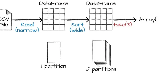
If we perform the take action on the DataFrame, we will be able to see the same results that we saw before when we used the command line:
flightData2015.take(3)
Array([United States,Romania,15], [United States,Croatia...
Let’s specify some more transformations! Now, let’s sort our data according to the count column, which is an integer type. Figure 2-8 illustrates this process.
Remember, sort does not modify the DataFrame. We use sort as a transformation that returns a new DataFrame by transforming the previous DataFrame. Let’s illustrate what’s happening when we call take on that resulting DataFrame (Figure 2-8).
Figure 2-8. Reading, sorting, and collecting a DataFrame
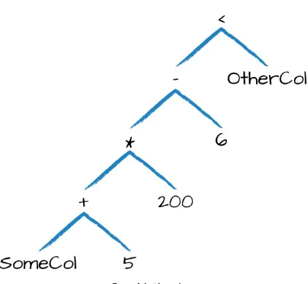
Nothing happens to the data when we call sort because it’s just a transformation. However, we can see that Spark is building up a plan for how it will execute this across the cluster by looking at the explain plan. We can call explain on any DataFrame object to see the DataFrame’s lineage (or how Spark will execute this query):
flightData2015.sort("count").explain()
== Physical Plan ==
*Sort [count#195 ASC NULLS FIRST], true, 0
+- Exchange rangepartitioning(count#195 ASC NULLS FIRST, 200)
+- *FileScan csv [DEST_COUNTRY_NAME#193,ORIGIN_COUNTRY_NAME#194,count#195] ...
Congratulations, you’ve just read your first explain plan! Explain plans are a bit arcane, but with a bit of practice it becomes second nature. You can read explain plans from top to bottom, the top being the end result, and the bottom being the source(s) of data. In this case, take a look at the first keywords. You will see sort, exchange, and FileScan. That’s because the sort of our data is actually a wide
transformation because rows will need to be compared with one another. Don’t worry too much about understanding everything about explain plans at this point, they can just be helpful tools for debugging and improving your knowledge as you progress with Spark.
Now, just like we did before, we can specify an action to kick off this plan. However, before doing that, we’re going to set a configuration. By default, when we perform a shuffle, Spark outputs 200 shuffle partitions. Let’s set this value to 5 to reduce the number of the output partitions from the shuffle:
spark.conf.set("spark.sql.shuffle.partitions","5")
flightData2015.sort("count").take(2)
... Array([United States,Singapore,1], [Moldova,United States,1])
the physical partition count, as well.
Figure 2-9. The process of logical and physical DataFrame manipulation
The logical plan of transformations that we build up defines a lineage for the DataFrame so that at any given point in time, Spark knows how to recompute any partition by performing all of the operations it had before on the same input data. This sits at the heart of Spark’s programming model—functional programming where the same inputs always result in the same outputs when the transformations on that data stay constant.
We do not manipulate the physical data; instead, we configure physical execution characteristics through things like the shuffle partitions parameter that we set a few moments ago. We ended up with five output partitions because that’s the value we specified in the shuffle partition. You can change this to help control the physical execution characteristics of your Spark jobs. Go ahead and
experiment with different values and see the number of partitions yourself. In experimenting with different values, you should see drastically different runtimes. Remember that you can monitor the job progress by navigating to the Spark UI on port 4040 to see the physical and logical execution
characteristics of your jobs.
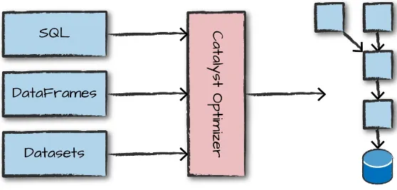
DataFrames and SQL
We worked through a simple transformation in the previous example, let’s now work through a more complex one and follow along in both DataFrames and SQL. Spark can run the same transformations, regardless of the language, in the exact same way. You can express your business logic in SQL or DataFrames (either in R, Python, Scala, or Java) and Spark will compile that logic down to an
You can make any DataFrame into a table or view with one simple method call:
flightData2015.createOrReplaceTempView("flight_data_2015")
Now we can query our data in SQL. To do so, we’ll use the spark.sql function (remember, spark is our SparkSession variable) that conveniently returns a new DataFrame. Although this might seem a bit circular in logic—that a SQL query against a DataFrame returns another DataFrame—it’s actually quite powerful. This makes it possible for you to specify transformations in the manner most
convenient to you at any given point in time and not sacrifice any efficiency to do so! To understand that this is happening, let’s take a look at two explain plans:
// in Scala
.groupBy('DEST_COUNTRY_NAME)
.count()
.groupBy("DEST_COUNTRY_NAME")\ .count()
+- *HashAggregate(keys=[DEST_COUNTRY_NAME#182], functions=[partial_count(1)]) +- *FileScan csv [DEST_COUNTRY_NAME#182] ...
== Physical Plan ==
*HashAggregate(keys=[DEST_COUNTRY_NAME#182], functions=[count(1)]) +- Exchange hashpartitioning(DEST_COUNTRY_NAME#182, 5)
+- *HashAggregate(keys=[DEST_COUNTRY_NAME#182], functions=[partial_count(1)]) +- *FileScan csv [DEST_COUNTRY_NAME#182] ...
Let’s pull out some interesting statistics from our data. One thing to understand is that DataFrames (and SQL) in Spark already have a huge number of manipulations available. There are hundreds of functions that you can use and import to help you resolve your big data problems faster. We will use the max function, to establish the maximum number of flights to and from any given location. This just scans each value in the relevant column in the DataFrame and checks whether it’s greater than the previous values that have been seen. This is a transformation, because we are effectively filtering down to one row. Let’s see what that looks like:
spark.sql("SELECT max(count) from flight_data_2015").take(1) // in Scala
importorg.apache.spark.sql.functions.max
flightData2015.select(max("count")).take(1) # in Python
frompyspark.sql.functions importmax
flightData2015.select(max("count")).take(1)
Great, that’s a simple example that gives a result of 370,002. Let’s perform something a bit more complicated and find the top five destination countries in the data. This is our first
| United States| 411352|
Now, let’s move to the DataFrame syntax that is semantically similar but slightly different in implementation and ordering. But, as we mentioned, the underlying plans for both of them are the same. Let’s run the queries and see their results as a sanity check:
// in Scala
importorg.apache.spark.sql.functions.desc
flightData2015
.groupBy("DEST_COUNTRY_NAME")
.sum("count")
.withColumnRenamed("sum(count)","destination_total")
.sort(desc("destination_total"))
.groupBy("DEST_COUNTRY_NAME")\ .sum("count")\
.withColumnRenamed("sum(count)", "destination_total")\ .sort(desc("destination_total"))\
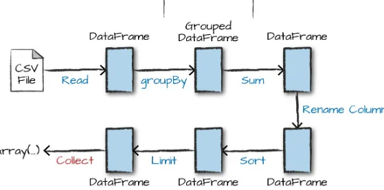
Figure 2-10. The entire DataFrame transformation flow
The first step is to read in the data. We defined the DataFrame previously but, as a reminder, Spark does not actually read it in until an action is called on that DataFrame or one derived from the original DataFrame.
The second step is our grouping; technically when we call groupBy, we end up with a
RelationalGroupedDataset, which is a fancy name for a DataFrame that has a grouping specified but needs the user to specify an aggregation before it can be queried further. We basically specified that we’re going to be grouping by a key (or set of keys) and that now we’re going to perform an
aggregation over each one of those keys.
Therefore, the third step is to specify the aggregation. Let’s use the sum aggregation method. This takes as input a column expression or, simply, a column name. The result of the sum method call is a new DataFrame. You’ll see that it has a new schema but that it does know the type of each column. It’s important to reinforce (again!) that no computation has been performed. This is simply another transformation that we’ve expressed, and Spark is simply able to trace our type information through it.
The fourth step is a simple renaming. We use the withColumnRenamed method that takes two arguments, the original column name and the new column name. Of course, this doesn’t perform computation: this is just another transformation!
The fifth step sorts the data such that if we were to take results off of the top of the DataFrame, they would have the largest values in the destination_total column.
actually the exact same thing.
Penultimately, we’ll specify a limit. This just specifies that we only want to return the first five values in our final DataFrame instead of all the data.
The last step is our action! Now we actually begin the process of collecting the results of our DataFrame, and Spark will give us back a list or array in the language that we’re executing. To reinforce all of this, let’s look at the explain plan for the previous query:
// in Scala
flightData2015
.groupBy("DEST_COUNTRY_NAME")
.sum("count")
.withColumnRenamed("sum(count)","destination_total")
.sort(desc("destination_total"))
.limit(5)
.explain() # in Python
flightData2015\
.groupBy("DEST_COUNTRY_NAME")\ .sum("count")\
.withColumnRenamed("sum(count)", "destination_total")\ .sort(desc("destination_total"))\ +- Exchange hashpartitioning(DEST_COUNTRY_NAME#7323, 5)
+- *HashAggregate(keys=[DEST_COUNTRY_NAME#7323], functions=[partial_sum... +- InMemoryTableScan [DEST_COUNTRY_NAME#7323, count#7325L]
+- InMemoryRelation [DEST_COUNTRY_NAME#7323, ORIGIN_COUNTRY_NA... +- *Scan csv [DEST_COUNTRY_NAME#7578,ORIGIN_COUNTRY_NAME...
Although this explain plan doesn’t match our exact “conceptual plan,” all of the pieces are there. You can see the limit statement as well as the orderBy (in the first line). You can also see how our
aggregation happens in two phases, in the partial_sum calls. This is because summing a list of
numbers is commutative, and Spark can perform the sum, partition by partition. Of course we can see how we read in the DataFrame, as well.
Naturally, we don’t always need to collect the data. We can also write it out to any data source that Spark supports. For instance, suppose we want to store the information in a database like PostgreSQL or write them out to another file.
Conclusion
Chapter 3. A Tour of Spark’s Toolset
In Chapter 2, we introduced Spark’s core concepts, like transformations and actions, in the context of Spark’s Structured APIs. These simple conceptual building blocks are the foundation of Apache Spark’s vast ecosystem of tools and libraries (Figure 3-1). Spark is composed of these primitives— the lower-level APIs and the Structured APIs—and then a series of standard libraries for additional functionality.
Figure 3-1. Spark’s toolset
Spark’s libraries support a variety of different tasks, from graph analysis and machine learning to streaming and integrations with a host of computing and storage systems. This chapter presents a whirlwind tour of much of what Spark has to offer, including some of the APIs we have not yet
This chapter covers the following:
Running production applications with spark-submit Datasets: type-safe APIs for structured data
Structured Streaming
Machine learning and advanced analytics
Resilient Distributed Datasets (RDD): Spark’s low level APIs SparkR
The third-party package ecosystem
After you’ve taken the tour, you’ll be able to jump to the corresponding parts of the book to find answers to your questions about particular topics.
Running Production Applications
Spark makes it easy to develop and create big data programs. Spark also makes it easy to turn your interactive exploration into production applications with spark-submit, a built-in command-line tool. spark-submit does one thing: it lets you send your application code to a cluster and launch it to
execute there. Upon submission, the application will run until it exits (completes the task) or encounters an error. You can do this with all of Spark’s support cluster managers including Standalone, Mesos, and YARN.
spark-submit offers several controls with which you can specify the resources your application needs as well as how it should be run and its command-line arguments.
You can write applications in any of Spark’s supported languages and then submit them for execution. The simplest example is running an application on your local machine. We’ll show this by running a sample Scala application that comes with Spark, using the following command in the directory where you downloaded Spark:
./bin/spark-submit \
--class org.apache.spark.examples.SparkPi \ --master local \
./examples/jars/spark-examples_2.11-2.2.0.jar 10
This sample application calculates the digits of pi to a certain level of estimation. Here, we’ve told spark-submit that we want to run on our local machine, which class and which JAR we would like to run, and some command-line arguments for that class.
We can also run a Python version of the application using the following command:
--master local \
./examples/src/main/python/pi.py 10
By changing the master argument of spark-submit, we can also submit the same application to a cluster running Spark’s standalone cluster manager, Mesos or YARN.
spark-submit will come in handy to run many of the examples we’ve packaged with this book. In the rest of this chapter, we’ll go through examples of some APIs that we haven’t yet seen in our
introduction to Spark.
Datasets: Type-Safe Structured APIs
The first API we’ll describe is a type-safe version of Spark’s structured API called Datasets, for writing statically typed code in Java and Scala. The Dataset API is not available in Python and R, because those languages are dynamically typed.
Recall that DataFrames, which we saw in the previous chapter, are a distributed collection of objects of type Row that can hold various types of tabular data. The Dataset API gives users the ability to assign a Java/Scala class to the records within a DataFrame and manipulate it as a collection of typed objects, similar to a Java ArrayList or Scala Seq. The APIs available on Datasets are type-safe, meaning that you cannot accidentally view the objects in a Dataset as being of another class than the class you put in initially. This makes Datasets especially attractive for writing large applications, with which multiple software engineers must interact through well-defined interfaces.
The Dataset class is parameterized with the type of object contained inside: Dataset<T> in Java and Dataset[T] in Scala. For example, a Dataset[Person] will be guaranteed to contain objects of class Person. As of Spark 2.0, the supported types are classes following the JavaBean pattern in Java and case classes in Scala. These types are restricted because Spark needs to be able to automatically analyze the type T and create an appropriate schema for the tabular data within your Dataset.
One great thing about Datasets is that you can use them only when you need or want to. For instance, in the following example, we’ll define our own data type and manipulate it via arbitrary map and filter functions. After we’ve performed our manipulations, Spark can automatically turn it back into a DataFrame, and we can manipulate it further by using the hundreds of functions that Spark includes. This makes it easy to drop down to lower level, perform type-safe coding when necessary, and move higher up to SQL for more rapid analysis. Here is a small example showing how you can use both type-safe functions and DataFrame-like SQL expressions to quickly write business logic:
// in Scala
case class Flight(DEST_COUNTRY_NAME:String,
ORIGIN_COUNTRY_NAME:String,
count:BigInt) valflightsDF=spark.read
One final advantage is that when you call collect or take on a Dataset, it will collect objects of the proper type in your Dataset, not DataFrame Rows. This makes it easy to get type safety and securely perform manipulation in a distributed and a local manner without code changes:
// in Scala
flights
.filter(flight_row=>flight_row.ORIGIN_COUNTRY_NAME!="Canada")
.map(flight_row=>flight_row)
.take(5)
flights
.take(5)
.filter(flight_row=>flight_row.ORIGIN_COUNTRY_NAME!="Canada")
.map(fr=>Flight(fr.DEST_COUNTRY_NAME,fr.ORIGIN_COUNTRY_NAME,fr.count+5))
We cover Datasets in depth in Chapter 11.
Structured Streaming
Structured Streaming is a high-level API for stream processing that became production-ready in Spark 2.2. With Structured Streaming, you can take the same operations that you perform in batch mode using Spark’s structured APIs and run them in a streaming fashion. This can reduce latency and allow for incremental processing. The best thing about Structured Streaming is that it allows you to rapidly and quickly extract value out of streaming systems with virtually no code changes. It also makes it easy to conceptualize because you can write your batch job as a way to prototype it and then you can convert it to a streaming job. The way all of this works is by incrementally processing that data.
Let’s walk through a simple example of how easy it is to get started with Structured Streaming. For this, we will use a retail dataset, one that has specific dates and times for us to be able to use. We will use the “by-day” set of files, in which one file represents one day of data.
We put it in this format to simulate data being produced in a consistent and regular manner by a
different process. This is retail data so imagine that these are being produced by retail stores and sent to a location where they will be read by our Structured Streaming job.
It’s also worth sharing a sample of the data so you can reference what the data looks like:
InvoiceNo,StockCode,Description,Quantity,InvoiceDate,UnitPrice,CustomerID,Country
536365,85123A,WHITE HANGING HEART T-LIGHT HOLDER,6,2010-12-01 08:26:00,2.55,17... 536365,71053,WHITE METAL LANTERN,6,2010-12-01 08:26:00,3.39,17850.0,United Kin... 536365,84406B,CREAM CUPID HEARTS COAT HANGER,8,2010-12-01 08:26:00,2.75,17850...
// in Scala
valstaticDataFrame=spark.read.format("csv")
.option("header","true")
.option("inferSchema","true")
.load("/data/retail-data/by-day/*.csv")
staticDataFrame.createOrReplaceTempView("retail_data") valstaticSchema=staticDataFrame.schema
# in Python
staticDataFrame=spark.read.format("csv")\ .option("header", "true")\
.option("inferSchema", "true")\ .load("/data/retail-data/by-day/*.csv")
staticDataFrame.createOrReplaceTempView("retail_data")
staticSchema=staticDataFrame.schema
Because we’re working with time–series data, it’s worth mentioning how we might go along grouping and aggregating our data. In this example we’ll take a look at the sale hours during which a given customer (identified by CustomerId) makes a large purchase. For example, let’s add a total cost column and see on what days a customer spent the most.
The window function will include all data from each day in the aggregation. It’s simply a window over the time–series column in our data. This is a helpful tool for manipulating date and timestamps because we can specify our requirements in a more human form (via intervals), and Spark will group all of them together for us:
// in Scala
importorg.apache.spark.sql.functions.{window,column,desc,col}
staticDataFrame
.selectExpr(
"CustomerId",
"(UnitPrice * Quantity) as total_cost",
"InvoiceDate")
frompyspark.sql.functions importwindow, column, desc, col staticDataFrame\
.selectExpr( "CustomerId",
"(UnitPrice * Quantity) as total_cost", "InvoiceDate")\
.groupBy(
col("CustomerId"), window(col("InvoiceDate"), "1 day"))\ .sum("total_cost")\
It’s worth mentioning that you can also run this as SQL code, just as we saw in the previous chapter. Here’s a sample of the output that you’ll see:
+---+---+---+ |CustomerId| window| sum(total_cost)| +---+---+---+ | 17450.0|[2011-09-20 00:00...| 71601.44| ...
| null|[2011-12-08 00:00...|31975.590000000007| +---+---+---+
The null values represent the fact that we don’t have a customerId for some transactions.
That’s the static DataFrame version; there shouldn’t be any big surprises in there if you’re familiar with the syntax.
Because you’re likely running this in local mode, it’s a good practice to set the number of shuffle partitions to something that’s going to be a better fit for local mode. This configuration specifies the number of partitions that should be created after a shuffle. By default, the value is 200, but because there aren’t many executors on this machine, it’s worth reducing this to 5. We did this same operation in Chapter 2, so if you don’t remember why this is important, feel free to flip back to review.
spark.conf.set("spark.sql.shuffle.partitions","5")
Now that we’ve seen how that works, let’s take a look at the streaming code! You’ll notice that very little actually changes about the code. The biggest change is that we used readStream instead of read, additionally you’ll notice the maxFilesPerTrigger option, which simply specifies the number of files we should read in at once. This is to make our demonstration more “streaming,” and in a production scenario this would probably be omitted.
valstreamingDataFrame=spark.readStream
.schema(staticSchema)
.option("maxFilesPerTrigger",1)
.format("csv")
.option("header","true")
.load("/data/retail-data/by-day/*.csv") # in Python
streamingDataFrame=spark.readStream\ .schema(staticSchema)\
.option("maxFilesPerTrigger", 1)\ .format("csv")\
.option("header", "true")\
.load("/data/retail-data/by-day/*.csv")
Now we can see whether our DataFrame is streaming: