VARIANCE ANALYSIS AND COMPARISON IN COMPUTER-AIDED DESIGN
Torsten Ullricha, Thomas Schifferb, Christoph Schinkob, Dieter W. Fellnera,b,c
aFraunhofer Austria Research, Visual Computing Division, Graz, Austria bInstitut f¨ur ComputerGraphik und WissensVisualisierung, TU Graz, Austria c
Fraunhofer Institut f¨ur Graphische Datenverarbeitung & Technische Universit¨at Darmstadt, Germany
Inffeldgasse 16c, A-8010 Graz, Austria
KEY WORDS:
Computer-Aided Design, Cultural Hertiage, Heightfield, Offset Geometry, Ray Tracing/Ray Casting, Reverse Engineering, Visualiza-tion
ABSTRACT:
The need to analyze and visualize differences of very similar objects arises in many research areas: mesh compression, scan alignment, nominal/actual value comparison, quality management, and surface reconstruction to name a few. In computer graphics, for example, differences of surfaces are used for analyzing mesh processing algorithms such as mesh compression. They are also used to validate reconstruction and fitting results of laser scanned surfaces. As laser scanning has become very important for the acquisition and preservation of artifacts, scanned representations are used for documentation as well as analysis of ancient objects. Detailed mesh comparisons can reveal smallest changes and damages. These analysis and documentation tasks are needed not only in the context of cultural heritage but also in engineering and manufacturing. Differences of surfaces are analyzed to check the quality of productions.
Our contribution to this problem is a workflow, which compares a reference / nominal surface with an actual, laser-scanned data set. The reference surface is a procedural model whose accuracy and systematics describe the semantic properties of an object; whereas the laser-scanned object is a real-world data set without any additional semantic information.
1 INTRODUCTION
Measuring and analyzing differences between surfaces is a nec-essary task in many fields of research. These techniques are used, for example, to validate reconstruction and fitting results of laser scanned surfaces. As laser scanning has become very important for the acquisition and preservation of artifacts, scanned represen-tations are used for documentation as well as analysis of ancient objects. Detailed mesh comparisons can reveal smallest changes and damages. These analysis and documentation tasks are needed – not only in the context of cultural heritage but also in engineer-ing and manufacturengineer-ing: differences of surfaces are analyzed to check the quality of productions.
The current methods to describe the shape of three-dimensional objects can be classified into two groups: composition of primi-tives and procedural description. As a 3D acquisition device re-turns an agglomeration of elementary objects (e.g. a laser scanner returns points) the real-world data set is always a composition of primitives. The nominal surface including its semantic informa-tion is a CAD model. In many cases, the nominal surface is a procedural model as they represent an ideal object rather than a real one. As the enrichment of measured data with an ideal de-scription enhances the range of potential applications, the bridge between both the generative and the explicit geometry descrip-tion is very important. It combines the accuracy and systematics of generative models with the realism and the irregularity of real-world data. This connection is a great challenge as pointed out in “Procedural methods for 3D reconstruction” by David Arnold (Arnold, 2006).
2 SYSTEM ARCHITECTURE
The presented system performs a variance analysis on a reference mesh and a scanned mesh. It consists of three main parts.
1. Registration: The first step registers a generative model (including its free parameters) to a laser scan. A genera-tive model can be regarded as a functionM, which gener-ates geometry if called with parametersx. The registration step takesM and determines a parameter setx0, such that M(x0)fits a given scanS.
2. Variance analysis: The difference between the generative modelM(x0)and the laser scanS can be computed
effi-ciently using state-of-the-art ray tracing techniques.
3. Variance visualization and documentation:The obtained variance is visualized using X3D technology. An X3D file is generated containing the generative modelM(x0), a
tex-ture of distance values and shader code capable of applying the difference as displacements. This allows switching se-lectively between the two models or displaying both of them simultaneously.
3 REGISTRATION
A generative model does not store an object’s geometry (control points, vertices, faces, etc.) but a sequence of operators and pa-rameters in order to create it (Ullrich et al., 2010a). All models with well organized structures and repetitive forms benefit from procedural model descriptions. In these cases generative mod-eling is superior to conventional approaches. Its strength lies in a compact description, which does not depend on the counter of primitives but on the model’s complexity itself. As a result es-pecially large scale models and scenes can be created efficiently which has promoted generative modeling within the last few years. Another advantage of procedural modeling techniques is the in-cluded expert knowledge within an object description; e.g. clas-sification schemes used in architecture, civil engineering, etc. can be mapped to procedures. For a specific object only its type and its instantiation parameters are needed to create an instance. In this way generative modeling techniques are the perfect basis to encode procedural knowledge sematically (Schinko et al., 2010).
Reverse engineering forms the link between recording techniques on the one hand and modeling, markup, and indexing on the other hand (Ullrich et al., 2010b). The algorithm used in this first step has been presented in “Semantic Fitting and Reconstruc-tion” (Ullrich et al., 2008). It simply regards a generative script as a functionMwith input parametersx∈Rk. These parameters may have a semantic meaning (width, height, etc.). The regis-tration respectively the parameter estimation is based on classical minimization of an error function
f(x1, . . . , xk) = In this equation the laser-scanned, input data set is represented by a point cloudS ={s0, . . . , sn}. The optimization algorithm determines some instance parametersxso that as many points as possible are close to the corresponding model instanceM(x); i.e. the sum of distancesdbetween points and model instance is min-imal. In order to eliminate a disproportionate effect of outlying points an additional weighting function
ψ(x) = 1−e−x2/σ2 (2)
is used. The additional parameterσ should correspond to the noise level of the input data set. An adequateσensures that points whose distance to a model is±εhave only a small contribution to the error function. The heuristic to selectσsuch that a point with distancedand noiseεwill be weightedψ(d+ε) = 1/2,
yields good results.
A numerical optimization evaluates the generative script up to several thousand times. Therefore, we integrated a compiler which translates the script code to machine code (Schinko et al., 2010), (Strobl et al., 2010). The compiler parses the script, creates an abstract syntax tree and differentiates it with respect to input pa-rameters; i.e. the complete generative model descriptionM (in-cluding all possibly called subroutines) is differentiated with re-spect to its input parameters. As a consequence, the optimization can use both the objective function
f(x1, . . . , xk) =
n X
j=0
ψ(d(M(x1, . . . , xk), si)) (3)
as well as its partial derivatives∂x∂fi. This differentiating compiler offers the possibility to use gradient-based optimization routines in the first place. Without partial derivatives many numerical op-timization routines cannot be used at all or in a limited way.
As the distance computation is by far the most time-consuming
part of this algorithm, it uses geometrical, spatial hashing to speed up the cimputation. Due to the fact that the weighting functionψ
has an upper limit
∀x∈R : ψ(x)<1 (4)
and converges relatively fast to one the objective function can be evaluated very efficiently. The weighted distances of points “far away” (depending on a threshold calculated usingσ) can be approximated byψ≈1and do not have to be calculated exactly. Only small distances are evaluated exactly.
4 ACCELERATION STRUCTURE CONSTRUCTION
To speed up the ray intersection queries, we organize our laser-scanned triangle data in a special manner. In a first step, we en-close each triangle with an axis-aligned bounding box (AABB). By grouping AABBs recursively, a tree like structure is obtained. This kind of hierarchy is called bounding volume hierarchy (BVH) and is a very popular acceleration structure for ray tracing (see (Wald et al., 2007)). The BVH construction can be performed fully automatically using a recursive, top-down algorithm out-lined in Algorithm 1.
Algorithm 1Recursive, Top-Down Construction of the Bound-ing Volume Hierarchy. The geometry is partioned accordBound-ing to a cost function and the bounding volume of each node is updated accordingly.
1: procedureBUILDBVH(BVHNodenode) 2: ifNEEDSPLIT( )then
3: SPLITGEOMETRY( ) 4: BUILDBVH(Lef tChild) 5: BUILDBVH(RightChild)
6: COMPUTEAABB(Lef tChild,RightChild) 7: else
8: COMPUTEAABB(objects) 9: end if
10: end procedure
We use a binary BVH, where each node has two child nodes max-imum (called left and right child). The construction is invoked for the root node of the BVH, which is passed all triangles of the in-put mesh. If the geometry contained in a node needs to be split, it is partioned among the child nodes and construction proceeds recursively. Then, the node’s AABB has to be updated, either us-ing the child AABBs or the contained objects (if no split has been performed).
In our implementation, a node is split whenever it contains more than four triangles. Splitting itself is guided by the commonly used surface area heuristic (SAH) cost function. It states that, as-suming uniformly distributed rays, the probability of a ray inter-secting a child nodeCgiven that its parent nodePis intersected is proportional to the ratio of the surface areas of the bounding boxes as shown in Formula 5
P rob(ray hits C|ray hits P)∝surf aceArea(C.AABB)
surf aceArea(P.AABB). (5) We use Formula 6 proposed in (Wald, 2007), which is based on the SAH, to guide our object partioning step.
cost(L, R) =NLAL+NRAR (6)
intersection costs of a ray with the BVH by grouping suitable AABBs. To reduce the search space for partitions, the centroids of the AABBs are projected along each coordinate axis and sorted in ascending order. The partition with minimal costs can then be found by ”sweeping” a split plane along the axis (see also (Wald et al., 2007)). This is done for all three coordinate axes and the split with minimal costs is finally selected.
5 PARALLEL RAY TRACING
A previously constructed BVH can be traversed in depth-first or-der using Algorithm 2. This recursive approach traverses the nodes that are intersected by a ray in strict front-to-back order. To maintain this node odering, a stack per ray is required, to store intersected nodes for later use.
Algorithm 2Depth-First Traversal of the Bounding Volume Hi-erarchy (BVH). The recursive algorithm traverses the nodes of the BVH in a strict front-to-back order and test the geometry con-tained in the leaves for intersection.
1: procedureIINTERSECTBVH(Rayray, BVHNodenode) 2: ifnodeis a leafthen
3: INTERSECTTRIANGLES(ray) 4: else
5: tlef t←INTERSECTAABB(Lef tChild,ray) 6: tright←INTERSECTAABB(RightChild,ray) 7: iftlef tANDtrightthen
13: INTERSECTBVH(ray,RightChild)
14: end if
15: else
16: iftlef tthen
17: INTERSECTBVH(ray,Lef tChild) 18: else iftrightthen
19: INTERSECTBVH(ray,RightChild) 20: else
The traversal is started from the root node using the ray as param-eter. If the node is a leaf, the contained geometry is intersected with the ray and the ray parameters are updated. An inner node has two child nodes, which are both intersected with the ray. If both children are intersected, the child that is closer to the ray’s origin is traversed recursively first, while the farther one is pushed onto the stack. If just one of the children is intersected, traversal proceeds to this child immediately. When no child node was in-tersected, a node is popped from the stack and traversal continues. The intersection search stops, if the stack gets empty and no more nodes are left for traversal. This depth-first order traversal can be used to find an ray intersection inO(log(N))time on average, instead of the naiveO(N)(Ndenotes the number of triangles).
To trace millions of rays in parallel, we implemented the depth-first traversal on the GPU using NVidia’s CUDA technology (see
(Lindholm et al., 2008) and (NVIDIA, 2010)). As mentioned be-fore, the constructed BVH is transferred to GPU memory, where it is subsequently traversed in massively parallel fashion. We use the approach of Aila et al. (Aila and Laine, 2009), which maps one ray to one thread. All threads execute our implementation of Algorithm 2 to find their intersection points.
6 DISTANCE CALCULATION AND ENCODING
The distance values for visualization and documentation purposes are obtained in a pre-processing step. A tool expects the reference model as well as the scanned model as input. Both models are en-coded in common 3D formats such as Alias / WaveFront object (.obj) or 3D Systems stereolithography (.stl) in order to be recog-nized by our importer. Once the mesh data is available, the ray casting library is initialized with the scanned model.
The next step is to obtain vertices and the corresponding normals on the reference mesh to start casting rays. A trivial approach would be to just use the vertices and normals supplied by the im-porter. By analyzing a typical mesh with texture coordinates one can easily see why this approach would be a waste of resources. Texture coordinates seldomly degenerate to one single (u,v) co-ordinate for all vertices defining a primitive - may it be a triangle or a quad. Therefore it is meaningful to not only use the texels as-sociated with the vertices defining the primitives to store the dis-tance values, but to use all texels inside the primitive. To fill the texels with distance values it is necessary to obtain position and normal in object coordinates. This is an easy task at the border texels of the primitive - since these values are available directly, but involves calculating object coordinates out of texel values for all other texels.
After obtaining all texels covered by the primitive, the corre-sponding object coordinates are calculated. These coordinates together with two vectors, one in positive and one in negative nor-mal direction of the primitive, represent rays to be tested against the scanned model. The ray casting library calculates the inter-section points - if there are any - up to a predefined maximum distance. The next step is to encode the distance values in a tex-ture following a pre-defined scheme. We store the distance of a hit in positive and negative direction as unsigned byte in the red, respectively green channel of the texture. The blue channel is used to encode the available distance information:
• A value of 0 means there is no hit in positive or negative direction.
• If there is a hit in negative direction, the value of 64 is added.
• In case there is a hit in positive direction, the value of 128 is added.
For an example distance texture please see Figure 1.
The texture encoding allows to carry out a selective displacement in the geometry shader incorported in the output X3D (Web3D Con-sortium, 2003) file. A built-in exporter creates the X3D file which we describe in detail in the next paragraph.
7 VISUALIZATION AND DOCUMENTATION
Figure 1: This distance texture is used in a displacement shader to create an output mesh which ideally matches a target mesh. Three color channels are used to encode distance values. The red and green channels are used to store distance values, whereas the blue channel is used to store additional information.
prefer a commonly used framework - which we found in X3D. For documentation purposes, the X3D solution offers an inte-grated, standard compliant approach to visualize both, the gener-ative as well as the laser-scanned model. Furthermore, the stan-dardized X3D format meets most documentation requirements. The generated X3D file incorporates the following components:
• The geometry of the reference mesh as indexed face set,
• a texture storing distance values to the scanned mesh
• as well as vertex, geometry and fragment shaders for dis-placement and lighting purposes.
The reference mesh and the distance texture represent the input for the shader stages. The vertex shader primarily acts as a pass-through stage. Position, normal and texture coordinates of the in-put vertex are handed over to the geometry shader for further pro-cessing. The geometry shader accepts triangles as input and out-put type. For each inout-put vertex, a texture lookup reveals whether the vertex needs to be displaced. In case there is a distance value in the texture, the displacement of the 3 vertices is calulated and an output triangle is generated. When distance values in positive and negative direction are available, two triangles are emitted. In all other cases there is no output at all. Additionally the shader allows to recursively subdivide input triangles to meet the desired output resolution of one vertex for almost every texel. This way we obtain a good representation of the scanned mesh. As a last stage, Blinn-Phong lighting is carried out on a per pixel basis in the fragment shader.
8 RESULTS AND DISCUSSION
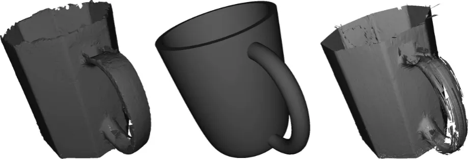
To demonstrate our workflow we use an example data set, which consists of a laser-scanned cup and a generative reference model.
The laser scan has 66 243 vertices and 130 973 faces (triangles). As the real cup has a clean and shiny surface, it has been difficult
to scan. The scan result is noisy and its not-cleaned-up mesh (mesh reparing, hole filling, mesh smoothing has not been done) has many holes (see Figure 3 (left)).
The generative cup model takes 15 parameters: (x, y, z)is the base point of the cup and (α, β, γ) define its orientation. Its shape is defined by an innerfin(x) = 1
25(x+ 1 10)
2+shape and outerfout(x) =x3+shapeshape function with one free parame-tershape. These functions are rotated around the cup’s main axis and scaled with the parametersrandh. The handle is defined via six parameters, which form points in 2D (in the plane of the handle, which is defined implicitly by its orientationγ); namely (h1, fout(h1)),(h2A, h2B),(h3A, h3B), and(h4, fout(h4)). They
are the control points of a B´ezier curve. Its tube with a fixed di-ameter (10mm) defines the cup’s handle.
The registration and optimization routines of the first step of our piepline determine the best-fit parameters automatically. The re-sult is shown in Figure 3 (middle).
The next step performs the variance analysis and stores its result in a texture map. The distance values are:
average distance 2.9613 mm maximum distance 8.6856 mm standard deviation 1.9820 mm
The per-texel-distances are visualized in Figure 2. As the gener-ative cup is rotationally symmetric, and the laser-scanned has an octagonal footprint, the distance map shows eight repetitions of (more or less) the same pattern. Furthermore, the starting-points of the handle can be identified clearly. The texture of the handle itself is on the right-hand-side of the texture map.
Figure 2: This is the distance texture of a cup with an orthogonal footprint. One can identify eight repetitions of (more or less) the same pattern.
9 CONCLUSIONS AND FUTURE WORK
Figure 3: This figure shows the scanned model (left), the reference model (middle), as well as the output of the variance visualization (right). The reference model is defined by a set of parameters obtained in a fitting process applied on the scanned model. A subsequent variance analysis leaves us with a X3D file capable of displacing the reference mesh to match the scanned mesh as good as possible.
the laser-scanned data set. An efficient ray intersection algorithm is used to obtain distance values between sample points on the reference surface and the scanned surface. These distance values are encoded in a texture and exported together with the refer-ence mesh as X3D file. An embedded displacement shader gen-erates a mesh resulting in a good representation of the actual, laser-scanned data set.
However there are some deficiencies in the output mesh since we are displacing the vertices in normal direction. Depending on the curvature of the surface we have to deal with gaps or overlaps. This could be fixed by taking the adjacent primitives into account and displacing the vertices in averaged normal direction.
Another aspect are artifacts or holes in the scanned surface which may produce unwanted results. This could probably be fixed in a pre-processing step. Still an open question is how to deal with scan data that has no correspondence in the generative model at all. We can deal with this kind of problem by adjusting the max-imum allowed distance value, but this leaves us with no output geometry for that part of the scan data.
ACKNOWLEDGEMENTS
The authors gratefully acknowledge the generous support from the European Commission for the integrated project 3D-COFORM (3D COllection FORMation, www.3D-coform.eu) under grant number FP7 ICT 231809.
We would also like to thank the Austrian Research Promotion Agency (FFG) for the research project METADESIGNER (Meta-Design Builder: A framework for the definition of end user inter-faces for product mass-customization), grant number 820925 / 18236.
Additionally, the German Research Foundation DFG for the re-search project PROBADO (PROtotypischer Betrieb Allgemeiner DOkumente, http://www.probado.de) supports this work under grant INST 9055/1-1.
Furthermore, part of our work is funded by the Doctoral Program Confluence of Vision and Graphics sponsored by the Austrian Science Fund (FWF).
REFERENCES
Aila, T. and Laine, S., 2009. Understanding the efficiency of ray traversal on gpus. In: Proceedings of the Conference on High
Performance Graphics 2009, HPG ’09, ACM, New York, NY, USA, pp. 145–149.
Arnold, D., 2006. Procedural methods for 3D reconstruction. Recording, Modeling and Visualization of Cultural Heritage 1, pp. 355–359.
Lindholm, E., Nickolls, J., Oberman, S. and Montrym, J., 2008. Nvidia tesla: A unified graphics and computing architecture. Mi-cro, IEEE 28(2), pp. 39 –55.
NVIDIA, 2010. NVIDIA CUDA Programming Manual 3.1.
Schinko, C., Strobl, M., Ullrich, T. and Fellner, D. W., 2010. Modeling Procedural Knowledge – a generative modeler for cul-tural heritage. Proccedings of EUROMED 2010 - Lecture Notes on Computer Science 6436, pp. 153–165.
Strobl, M., Schinko, C., Ullrich, T. and Fellner, D. W., 2010. Euclides – A JavaScript to PostScript Translator. Proccedings of the International Conference on Computational Logics, Algebras, Programming, Tools, and Benchmarking (Computation Tools) 1, pp. 14–21.
Ullrich, T., Schinko, C. and Fellner, D. W., 2010a. Procedural Modeling in Theory and Practice. Poster Proceedings of the 18th WSCG International Conference on Computer Graphics, Visual-ization and Computer Vision 18, pp. 5–8.
Ullrich, T., Settgast, V. and Berndt, R., 2010b. Semantic En-richment for 3D Documents: Techniques and Open Problems. Publishing in the Networked World: Transforming the Nature of Communication, Proceedings of the International Conference on Electronic Publishing 14, pp. 374–384.
Ullrich, T., Settgast, V. and Fellner, D. W., 2008. Semantic Fitting and Reconstruction. Journal on Computing and Cultural Heritage 1(2), pp. 1201–1220.
Wald, I., 2007. On fast construction of sah-based bounding vol-ume hierarchies. In: In Proceedings of the 2007 IEEE/EG Sym-posium on Interactive Ray Tracing. IEEE, pp. 33–40.
Wald, I., Mark, W. R., G¨unther, J., Boulos, S., Ize, T., Hunt, W., Parker, S. G. and Shirley, P., 2007. State of the art in ray tracing animated scenes. In: D. Schmalstieg and J. Bittner (eds), STAR Proceedings of Eurographics 2007, The Eurographics Associa-tion, pp. 89–116.