A new electric method for non invasive c

R E S E A R C H

Open Access

A new electric method for non-invasive

continuous monitoring of stroke volume and

ventricular volume-time curves

Maurits K Konings

*

, Henk G Goovaerts, Maarten R Roosendaal, Rienk Rienks, Ferry M Koevoets,

Ronald L Bleys, Wolfgang F Buhre, Paul M Dorresteijn, Tim Hesselink, Arthur E Officier, Charles L Hollenkamp

and Frank E Rademakers

*Correspondence: m.konings@umcutrecht.nl Dept. of Medical Technology, University Medical Center Utrecht, Utrecht, The Netherlands

Abstract

Background: In this paper a new non-invasive, operator-free, continuous ventricular stroke volume monitoring device (Hemodynamic Cardiac Profiler, HCP) is presented, that measures the average stroke volume (SV) for each period of 20 seconds, as well as ventricular volume-time curves for each cardiac cycle, using a new electric method (Ventricular Field Recognition) with six independent electrode pairs distributed over the frontal thoracic skin. In contrast to existing non-invasive electric methods, our method does not use the algorithms of impedance or bioreactance cardiography. Instead, our method is based on specific 2D spatial patterns on the thoracic skin, representing the distribution, over the thorax, of changes in the applied current field caused by cardiac volume changes during the cardiac cycle. Since total heart volume variation during the cardiac cycle is a poor indicator for ventricular stroke volume, our HCP separates atrial filling effects from ventricular filling effects, and retrieves the volume changes of only the ventricles.

Methods: ex-vivo experiments on a post-mortem human heart have been performed to measure the effects of increasing the blood volume inside the ventricles in isolation, leaving the atrial volume invariant (which can not be done in-vivo). These effects have been measured as a specific 2D pattern of voltage changes on the thoracic skin. Furthermore, a working prototype of the HCP has been developed that uses these ex-vivo results in an algorithm to decompose voltage changes, that were measured in-vivo by the HCP on the thoracic skin of a human volunteer, into an atrial component and a ventricular component, in almost real-time (with a delay of maximally 39 seconds). The HCP prototype has been tested in-vivo on 7 human volunteers, using G-suit inflation and deflation to provoke stroke volume changes, and LVot Doppler as a reference technique.

Results: The ex-vivo measurements showed that ventricular filling caused a pattern over the thorax quite distinct from that of atrial filling. The in-vivo tests of the HCP with LVot Doppler resulted in a Pearson’s correlation of R = 0.892, and Bland-Altman plotting of SV yielded a mean bias of -1.6 ml and 2SD=14.8 ml.

Conclusions: The results indicate that the HCP was able to track the changes in ventricular stroke volume reliably. Furthermore, the HCP produced ventricular volume-time curves that were consistent with the literature, and may be a diagnostic tool as well.

Background

In intensive care medicine, the measurement of left ventricular stroke volume (SV) and cardiac output (CO) is important in the hemodynamic management of peri-operative and critically ill patients. Pulmonary artery thermodilution CO monitoring using the pulmonary artery catheter has major disadvantages, because pulmonary artery catheter-ization is time-consuming, and associated with a risk of morbidity and mortality [1]. Noninvasive ultrasound Doppler techniques to determine CO have been developed, but require skilled operators, and therefore are not suited for monitoring CO continuously. More recently, esophageal Doppler, Fick principle applied to carbon dioxide, and pulse contour analysis have been identified as key technologies for cardiac output monitoring [2,3]. Furthermore, recent advances in MRI show promising results in measuring car-diac output [4,5]; MRI however is not suited for continuous bed-side monitoring. Stroke volume can also be measured reliably using the conductance catheter [6]. This method however requires a catheter to be placed in the left ventricle. The transcardiac conduc-tance method produces satisfactory results in a less invasive manner, but still requires an internal central venous electrode [7]. Thoracic impedance cardiography (ICG) is a non-invasive technique, but conflicting results concerning the validity and reliability of ICG have been reported, varying from satisfactory correlations [8-10] to poor correlations [11,12] in comparison to thermodilution CO measurements. Bioreactance cardiography [13] provides better results than ICG, because it measures also phase shifts instead of merely amplitudes of AC voltages, and bioreactance cardiography is currently being eval-uated in clinical settings. All in all however, there is still a need for a non-invasive, precise, continuous, and operator-free method of CO measurement.

Recently, such a method (which we will refer to as ’Ventricular Field Recognition’, VFR) has been developed in our group [14]. In a previous paper [15], we presented an animal study, in which the cardiac output readings using the new VFR method were compared to the cardiac output readings from a flow probe around the aorta, resulting in a bias of -0.114 L/minute and a variability of the bias (2 standard deviations, 2SD) of 0.55 L/minute in a Bland-Altman analysis; without however providing any mathematical details about the principle of operation of the new method. In the present paper, the physics and math-ematics of the principle of operation of the VFR method is presented, and some basic assumptions underlying the VFR method are analysed and investigated. Furthermore, we present the results of a validation study of the VFR method onhuman_volunteers.

The Ventricular Field Recognition method is based on our findings that, (i) if a weak, harmless, constant AC electric current is applied over the thorax, the emptying and filling of theventricles_{during the cardiac cycle gives rise to a specific two-dimensional spatial} pattern of changes in current density over the frontal thoracic skin during the cardiac cycle, and, furthermore, (ii) that this pattern is distinctly different from the spatial pattern of current density changes due to the filling and emptying of theatria_{. This is caused by} the fact that the ventricles are situated at other locations inside the thorax than the atria, and hence, the location (on the frontal thoracic skin) of the “ventricular epicenter” of the changes in the applied current field, due to ventricular volume changes, differs from the location of the “atrial epicenter” corresponding to atrial volume changes.

during the cardiac cycle, some atrial volume changes take place as well. Therefore, when measuring in-vivo on a patient or volunteer, the measured 2D pattern of voltage changes distributed over the skin of the thorax, is a superposition of three different patterns, viz. (i) the pattern due to volume changes in the atria, (ii) the pattern due to volume changes in the ventricles, and (iii) a pattern due to extracardial effects, such as e.g. diameter changes in large blood vessels outside the heart. In order to monitor the stroke volume and ven-tricular volume-time curves of a patient however, the volume changes in exclusively the ventricles have to be established (because total heart volume variation is a poor indicator of ventricular stroke volume [16]). Therefore, the Ventricular Field Recognition method presented in this paper has been designed to distill the ventricular volume changes from the measured total superposition of the three patterns. In order to do so, the specific pat-tern of voltage changes on the frontal thoracic skin associated with volume change inonly the ventricles, needs to be known.

Therefore, an extensive set ofex-vivomeasurements has been performed in our group, usingpost-mortemhuman hearts and thoraces. The valves inside the post-mortem human hearts were sealed, and each compartment of the heart was connected to a silicon tube leading to a large syringe, thus enabling the separate filling (or emptying) of e.g.only the ventricles, oronlythe atria, as will be explained in more detail in section Methods: ex-vivo post-mortem calibration. The effect of the filling action on the applied thoracic current density distribution was registered by a matrix of electrodes on the skin of the post-mortem thorax. In this way, a distinct 2D pattern on the frontal thoracic skin was measured, representing the voltage changes due to a specific standardized filling action of only the ventricles with a fixed known volume. We will refer to this specific spatial 2D pattern as the “ventricular fingerprint”. Furthermore, we measured an “atrial fingerprint” as well, representing a standardized filling of only the atria. Throughout this paper, the word “fingerprint” refers to the measurements performedex-vivoon humanpost-mortem cadaveric materials.

In thein-vivosituation, with a beating heart inside the thorax of a patient, the actual voltage change pattern that is measured over the frontal thoracic skin, is a linear combi-nation of thesepost-mortemventricular and atrial fingerprints, because volume changes take place in ventriclesandatria simultaneously during a cardiac cycle in-vivo. Let τ denote the time (in milliseconds), during one single cardiac cycle, that has lapsed after the last R-peak of the ECG. The above mentioned linear combination may then be written as:

in-vivo voltage(x_{,τ )}

−in-vivo voltage(x_{, 0)}

=α(τ )

atrial postmortem fingerprint(x₎

+ψ (τ )ventricular postmortem fingerprint(x₎

+noise (1)

in whichx_{denotes the coordinates of any point on the frontal thoracic skin, andα(τ )} andψ (τ )are time-dependent scalars. At the left side of the “equals” sign (“=”) in eq.(1) the in-vivo voltagechangeis defined as a subtraction, viz. the voltage at pointx_{at timeτ} during a specific cardiac cycleminusthe voltage at the same pointx_{at the beginning of} that same particular cardiac cycle (τ =0).

contributions from the atrial changes and the ventricular changes, respectively, to the total voltage change. The key point in our method is thatα(τ ) is a measure of atrial volume change, andψ (τ )is a measure of ventricular volume change (as will be shown in section Principle of Operation), at that particular instantτ during the cardiac cycle. Therefore, the graph ofψ (τ )as function of time during one single specific heartbeat rep-resents the in-vivo ventricular volume-time curve during that single specific heartbeat in a patient or volunteer. In this paper we will show that, if a sufficiently large number of voltage measuring electrodes is distributed over the thorax, and if the standardized, time-independentex-vivo post-mortematrial and ventricular fingerprints are known, then the values of the coefficientψ (τ )(during any cardiac cycle) during anin-vivomeasurement on a human volunteer, can be retrieved in a reliable manner on basis of thein-vivo mea-surement data at the left side of eq. (1), i.e. on basis of the voltage changes measured in-vivo on the thoracic skin of the volunteer. In other words, the in-vivo volume-time curveψ (τ )of a specific cardiac cycle of a patient can be solved from eq. (1), using the volt-age changes measured in-vivo on the thoracic skin of that patient, in combination with the standardized, generic, time-independentex-vivo post-mortematrial and ventricular fingerprints at the right side of eq. (1).

In our prototype, the Hemodynamic Cardiac Profiler (HCP, TM, pat. pend., [14]), we used seven thoracic voltage measuring electrodes distributed over the thoracic skin, com-bined into one single compound electrode sticker. These seven electrodes measured six independent voltage differences simultaneously. Our method isnotbased on impedance cardiography (ICG) algorithms, since we do not calculate any impedance measure, but use spatial patterns to retrieve volume changes of specifically the ventricles. Once the volume-time curveψ (τ )of a specific cardiac cycle is known, the ventricular stroke vol-ume (SV) of that specific cardiac cycle is known as well, because the stroke volvol-ume is calculated as the difference between the end-diastolic ventricular volume at the begin-ning of that particular cardiac cycle and the end-systolic ventricular volume of that cycle. Therefore, trend curves can be produced, consisting of large series of SV values of subse-quent cardiac cycles, representing the behavior of the SV over the course of minutes or hours.

Principle of Operation

In this section, it is explained (in subsection relative differential measurement) that the positions of the measuring electrodes and their connections to the voltage measuring electronics can be designed in such a way that the unwanted effects of other factors, such as e.g. the velocity-dependency of the conductivity of blood, or changes in the aortic diameter during the cardiac cycle, are minimized.

Subsequently, in subsection algorithm for retrieving ventricular volume-time curves and stroke volume, it is explained how the ψ (τ ) curve can be solved from eq.(1) on basis of the measured voltage change data in combination with the standardized (time-independent)ex-vivospatial atrial and ventricular fingerprints.

Relative differential measurement

The design of the multi-electrode configuration needed to be optimized for this task. Therefore, we formulated the following two demands, which were to be met by the multi-electrode configuration:

(i) insensitivity to conductivity changes or diameter changes, during each single cardiac cycle, within vertical elongated structures like the aorta or other larger blood vessels

(ii) insensitivity to thorax dimensions and other factors that influence the average, global, current strength inside the thorax.

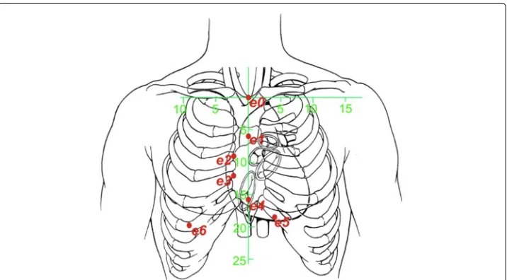
Demand (i) is met if the electrodes are placed in a vertical array over the central ster-nal line, and the voltages are measured between two adjacent electrodes with a relatively small inter-electrode distance. See the first five measuring electrodes (e0_toe4_{) in Figure 1.} (The other electrodes,e5_ande6_{, are placed to the left and the right of the vertical sternal} line, and used to deal with inter-patient anatomical differences, as explained later on). The measuring electrodes are numberede₀toe₆, and, for each value ofk(withk∈ {1. . .6}), the voltage(meask) is measured between the two electrodesek andek−1. This results in a measurement of an approximation of a vertical spatial “differential” of the voltage dis-tribution on the thoracic skin along the vertical sternal line. This “differential” along the vertical axis causes the measured voltage to be relatively insensitive to conductivity and diameter changes that are spread out in the vertical direction, as is the case with large vertical blood vessels.

Figure 1 Schematic rendering the electrode positions with respect to the anatomy of the human thorax.Distances printed along the green horizontal and vertical axes are in cm. In order to meet the demands (i) and (ii) in subsection relative differential measurement, the electrodes are distributed along the central vertical axis of the sternum. Furthermore, the electrodes spread out to the left and the right side of the thoraxbelowthe inframammary fold to enable application on female patients without disturbance from the mammae. The positions on the thoracic skin are defined using the green 2D coordinate system (x,z), of which the origin (x=0 andz=0) coincides with the position of the top end of the sternal bone, near the incisura jugularis. The measuring electrodes are numberede₀toe₆, and, for each value ofk(withk∈ {1. . .6}), the input voltage(meask) from eq.(2) is measured between the two electrodesekandek−1. The positions of

the seven electrodese₀toe₆are (in (x,z)-coordinates and in mm):

As has been indicated in the introduction, the basis of the input of our system is formed by the voltagechangesduring a specific cardiac cycle, as function of the timeτ (in mil-liseconds), with respect to the beginning of that cardiac cycle atτ = 0, in which the

beginning of a cardiac cycle (τ = 0) is defined as the moment in time when the R-peak of the ECG has its maximum. The measured voltage change between electrode pairk, as function ofτ, therefore reads:(k)meas(τ )−(k)meas(0).

Demand (ii) is met if subsequently this(k)meas(τ )−(k)meas(0)is divided by(k)meas(0)to

form a dimensionless numberϕmeas: ϕ_meas(k) (τ ) =

(k)meas(τ ) − (k)meas(0) (k)meas(0)

(2) As will be shown in the Appendix, the voltage change(k)meas(τ )−(k)meas(0)is

propor-tional to the strength of the incident applied current field near the heart. Furthermore, the(k)measitself is proportional to the incident applied current field (near electrodesek

andek−1), for all values ofτ (includingτ =0).

Therefore, the strength of the applied current is factored out due to the quotient in eq.(2), and the dimensionless numbersϕmeas(k) (τ )are insensitive to variations in applied

global current density.

Algorithm for retrieving ventricular volume-time curves and stroke volume

Inex-vivocalibration experiments on human postmortem hearts (to be described in more detail in section Methods: ex-vivo post-mortem calibration ), we measuredpostmortem_{ventric,before}

andpostmortem_{ventric,after}values on a post-mortem thorax, in whichpostmortem_{ventric,after} is measured after an artificial increase of the volume (with a known fixed standardized volumeVcalib) in

exclusively the ventricles of the post-mortem heart, andpostmortem_{ventric,before}is the initial value before the artificial increase.

Completely analogous to the definition of ϕmeas(k) in eq.(2), the (k)_ventric,postmortem_,before and (k)_ventric,postmortem_,after values are combined into a dimensionless scalarμ(k)_ventric,postmortem:

μ(k)_ventric,postmortem=

(k)_ventric,postmortem_,after −(k)_ventric,postmortem_,before

(k)_ventric,postmortem_,before

(3) in which the index(k)refers to exactly the same locations on the thorax as the positions of the electrodesekin thein-vivosituation in eq.(2).

These sixμ(k)_ventric,postmortemscalars are combined into a 6-dimensional “ventricular finger-print vector”f_V: (in which T indicates the transpose, switching between the horizontal and vertical nota-tion of a vector). Analogously, for ex-vivo post-mortem measurements of artificial filling of only the atria, we have the 6-dimensional “atrial fingerprint vector”f_A:

f_{A = μ}(1),postmortem Likewise, the ϕmeas values that are measured in-vivo on a patient (see eq.(2)), are

combined into a 6-dimensional measurement vectorv_meas: v_meas(τ ) =

ϕ_meas(1) (τ ),ϕ_meas(2) (τ ),· · ·,ϕmeas(6) (τ ) T

As has been indicated in the introduction using eq.(1), the ϕmeas values, measured in-vivo on a patient, are considered to be alinear combinationof the effects from the standard atrial ex-vivo post-mortem volume change (fingerprint vectorf_{A), and the} stan-dardized ventricular ex-vivo post-mortem volume change (fingerprint vectorf_{V). The} coefficients in this linear combination are the scalarsα(τ )andψ (τ ):

⎡

In order to retrieve the stroke volume and volume-time curves from the measured vmeas(τ ), the HCP has to solve the value of ψ (τ )from eq.(7) for each point in time

τ at which a measurement ofv_{meas has taken place (every 5 milliseconds in our HCP} prototype).

The last equation (eq. (7)), together with the method to solve the volume-time curves (ψ (τ )) from eq. (7) using the measured v_{meas(τ ), constitute the core of the new VFR} method presented in this paper.

Therefore, equation (7) has to be accounted for in the form of a fundamental physical reasoning that justifies this equation. This reasoning is provided in the Appendix (A1).

Furthermore, fundamentally speaking, any calculation of voltage changes on basis of volume changes of blood-filled lumina such as the ventricles, is anon-linearproblem. Therefore, the limits of the accuracy of this linear equation will be examined in the Appendix as well (in A2).

A method for retrievingψ (τ )from equation 7 is described directly below.

Given the possible presence of noise and artefacts, which are generally unrelated to the fingerprint patterns, the task for the real-time algorithm is to find the parametersα(τ ) andψ (τ )for which

|vmeas(τ ) − (α(τ )f_A+ψ (τ )f_V)| is minimal (8)

This task is performed by finding theα(τ )andψ (τ )that satisfy:

(v_meas(τ )−(α(τ )f_A+ψ (τ )f_V))·f_A = 0 (v_meas(τ )−(α(τ )f_A+ψ (τ )f_V))·f_V = 0

(9)

in which the inner product (“·”) between any two 6D-vectorsA_andB_{is defined} com-pletely analogously to the familiar 3-dimensional case, i.e.A · B = 6

α(τ ) = WA · vmeas(τ ) and ψ (τ ) = WV ·vmeas(τ ) (10)

in which

W_{A =} (fV · fV)fA − (fA · fV)fV (f_{A ·}f_A)(f_{V ·}f_{V) − (}f_{A ·} f_V)2

W_{V =} (fA · fA)fV − (fV · fA)fA

(f_{A ·}f_A)(f_{V ·}f_V) ₋ (f_{A ·} f_V)2 (11)

The “weight vectors”W_AandW_V are time-independent and completely based on only the ex-vivo “fingerprint” vectorsf_Aandf_{V. As a result, the}ψ (τ )is a linear function of the six measured voltages in thev_meas(τ )vector in eq.(10).

On basis of the results of the ex-vivo post-mortem calibration experiments (that will be described in section Methods: ex-vivo post-mortem calibration ), a fixed known standard ventricular volume increaseVcalibhas been linked to the “fingerprint vector”fV. There-fore, as an extreme and purely theoretical example, consider a case in which the volume of the atria would not change at all, and in which at some moment in timeτ, thev_meas(τ ) would be equal tof_{V. Then the value of}ψ (τ )would be equal to one (as can be seen in eq.(7)), and the ventricular volume changeV(τ )−V(0)(in whichV(τ )denotes the ven-tricular volume at timeτduring a specific cardiac cycle, andV(0)denotes the ventricular volume at the beginning (τ =0) of that specific cardiac cycle) would be equal toVcalibat timeτ.

In a realistic situation, in which the atrial and ventricular volumes change simultane-ously, we have (on basis of eq.(10)):

V(τ )− V(0) = ψ (τ )Vcalib = (vmeas(τ ) ·WV) Vcalib (12)

This equation constitutes the final result that has been implemented in the algorithm of the experimental prototype of the HCP, in order to calculate the ventricular volume-time curveV(τ )−V(0)from thevmeas(τ )measured in-vivo on volunteers.

Methods: ex-vivo post-mortem calibration

In order to perform realistic measurements ex-vivo, the front part of a post-mortem human thorax conserved in formalin was placed in a basin filled with a NaCl solution.

The concentration of the NaCl in the solution was such that the solution had a specific conductivity equal to the average conduction of thoracic tissue. The thorax was sus-pended halfway into the solution in such a way that the thoracic skin remained dry, but the rest of the thorax, including the curved inner side of the thoracic wall, was in direct contact with the NaCl solution.

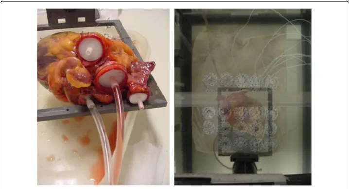
On the dry thoracic skin, a matrix of measuring electrodes was placed, in a two-dimensional array of 5×5 electrodes, with an interelectrode distance (as measured from the center of one electrode to the center of the next) of 35 mm in both the vertical and horizontal direction (see Figure 2). Each individual electrode from this 5 × 5 matrix was connected to a voltage measuring device, together with a reference measuring elec-trode that was placed centrally on the cranial ending of the sternum, in the middle of the incisura jugularis.

Figure 2left:Post-mortem human heart, with connecting tubes for the purpose of producing well-defined volume changes during the ex-vivo post-mortem calibration measurements as described in section Methods: ex-vivo post-mortem calibration.right:Experimental set-up with a postmortem human thorax, a post-mortem human heart, and a matrix of 5×5 measuring electrodes on the

skin of the postmortem human thorax. For visibility purposes, the thorax has been made semi-transparent in this image, in order to show the position of the heart lying underneath.

atria), it was essential that all heart valves within the heart were closed. Because of the fri-ability of the leaflets of the valves, patches of thin tissue were sutured over the orifice of the valves. The coronary arteries were ligatured at the root. In some cases, cyanoacrylate was used to seal a few small remaining leaks.

Measurements of the voltage field were made using the 2D electrode matrix, during fill-ing and emptyfill-ing of the different compartments of the heart. These compartments (atria and ventricles) were connected to plastic tubing and syringes (see left side of Figure 2) to enable controlled filling and emptying with a blood-equivalent NaCl solution. Plastic wire-straps were used to keep the tubing absolutely fixed and immobilized during the experiments. In order to let the heart retain a realistic shape during volume change of the ventricles, a simultaneous movement of two separate syringes was performed, filling the ventricles with 50 ml of blood-equivalent NaCl solution (having the same specific electric conductivity as blood), and simultaneously removing 50 ml of thorax-equivalent solution (i.e. a solution containing less NaCl, having the same average specific electric conductivity as the inside of the thorax) from the atria. This procedure caused the total heart volume to remain invariant. Furthermore, since the specific conductivity of the solution that was removed from the atria was equal to that of the solution outside the heart (viz. the thorax-equivalent solution), the electric effect of the volume decrease in the atria was annulled. At the same time however the electric effect of the volume decrease in the ventricles _was not _{annulled because the specific conductivity of the} removed blood-equivalent solution was much higher than that of the thorax-equivalent solution.

Since in the post-mortem ex-vivo measurements a post-mortem thorax was used, the post-mortem ex-vivo measurements were confined to the thoracic skin as well. No mea-surements were done ex-vivo on locations on the post-mortem skin that would have no in-vivo counterpart in the form of measurements on the same location on the skin in-vivo.

Methods: in-vivo tests of the HCP on volunteers

Experimental prototype of HCP

Respiration-gated algorithm

In order to exclude artefacts in the measured voltage change pattern (ϕ(k)meas withk ∈

{1, 2,. . ., 6}) on the thoracic skin due to distortions caused by changing air volumes inside the lungs, we adopted a respiration-gated approach. Preliminary measurements have shown that the absolute value of(k)meas(as opposed to the dimensionless relative

differ-enceϕmeas(k) ) is a reliable indicator of the volume of air inside the lungs. Therefore, by

monitoring the respiratory fluctuation in the series of absolute values ofmeas(0)from

subsequent heart cycles, the HCP automatically selects a subset of cardiac cycles, out of the total set of cardiac cycles within a period of 20 seconds, that corresponds to a spe-cific phase in the respiratory cycle (on basis of the trend in the series of(k)meas(0)values),

as well as to the same volume of air inside the lungs (on basis of the absolute value of (k)meas(0)values). In this way, this “-gated” algorithm serves as a respiration-gated

algo-rithm. This selection procedure on basis of the(k)meas(0) values takes place beforethe

algorithm (as specified in eq.(12)) is applied.

G-suit deflation, and LVot Doppler as a reference technique

In order to cause changes in stroke volume in volunteers, and at the same time let other (environmental) parameters remain the same as much as possible, we used inflatable anti-shock trousers (known as “G-suits” to air force pilots). Such antianti-shock trousers contain inflatable bladders inside the trousers. When inflated, these bladders produce pressure forces onto the legs, which prevent the blood to accumulate inside the legs when the airplane makes a sharp turn; hence these trousers prevent the pilot from loosing con-sciousness. It has been shown [19] that, in a standing position, sudden deflation of an inflated G-suit can cause the stroke volume to drop suddenly. We performed a procedure on 7 volunteers, in which a G-suit (Anti-G-Garment, CUTAWAY, CSU-13B/P, USAF, USA) was inflated gradually from 0 mmHg to 70 mmHg during 2 minutes and 30 sec-onds. Subsequently, a constant pressure of 70 mmHg pressure was maintained during 2 minutes, after which, finally, a sudden deflation back to 0 mmHg took place within 5 seconds.

The 7 volunteers were all healthy males, with a Body Mass Index ranging from nor-mal to slightly overweight. The volunteers had no visible abnornor-malities in their thoracic anatomy, and were randomly selected from the male population on the Utrecht Univer-sity Campus. All volunteers have read and signed an Informed Consent form, prior to the experiments. All procedures concerning the volunteers in this study have been exe-cuted in compliance with the guidelines of the University Medical Center Utrecht (and in compliance with the Helsinki Declaration), and have been approved by the Authority for Safety of the University Medical Center Utrecht.

volunteer’s heart rate. In the apical 5-chamber view the Pulsed Wave Doppler sample vol-ume was positioned about 0.5 cm proximal of the Aorta-valve in line with the blood flow direction as indicated by the color Doppler. This position was regularly checked, depend-ing on the movements of the volunteer. The LVot area was calculated usdepend-ing the measured LVot diameter, average of 2 measurements, in a enlarged view of the Aorta-valve in the para-sternal long axes view.

This validation focussed on investigating the capability of monitoring changes in SV during de G-suit manipulations correctly. For each individual volunteer, a single and con-stant scaling factorKvolunteer was applied to the SV readings to let the average initial SV from the HCP coincide with the SV from the LVot Doppler.

Results

results of the ex-vivo post-mortem calibration

For each of the electrodes in the electrode matrix shown in Figure 2, the voltages postmortem_{ventric,before}andpostmortem_{ventric,after}have been measured, as well as the voltagespostmortem_{atrial,before}and

postmortem_atrial,after , in which “before” and “after” refer to the moment in time with respect to the artificial filling procedure. All voltages were measured with respect to a reference electrode at the incisura jugularis (not shown in the figures). Two-dimensional linear interpolation has been used to create the continuous two-dimensional interpolations postmortem_{ventric,before}(x,z) andpostmortem_{ventric,after}(x,z), as well aspostmortem_{atrial,before}(x,z)andpostmortem_atrial,after (x,z) from the discrete sets of measurements from the electrode matrix, in which the origin (x=0 and z=0) coincides with the position of the top end of the sternal bone, near the incisura jugularis, andxandzdenote the horizontal and vertical position with respect to the origin, respectively.

Whereas in eq.3 theμvalues were defined only for the 7 positions on the thorax on which the 7 electrodes (e0toe6) were located, we now define a similar value for each point (x,z) on the thoracic skin, in complete analogy to eq.3, using the above mentioned, exper-imentally obtained, interpolations postmortem_{ventric,before}(x,z), _{ventric,after}postmortem(x,z), postmortem_{atrial,before}(x,z)

andpostmortem_atrial,after (x,z):

mpostmortem_ventric (x,z)=

postmortem_{ventric,after}(x,z)−postmortem_{ventric,before}(x,z)

postmortem_{ventric,before}(x,z−15)−postmortem_{ventric,before}(x,z+15) (13)

and

mpostmortem_atrial (x,z)=

postmortem_atrial,after(x,z)−postmortem_{atrial,before}(x,z)

postmortem_{atrial,before}(x,z−15)−postmortem_{atrial,before}(x,z+15) (14)

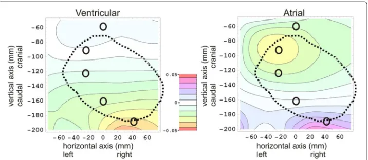
The 2D color contour plots ofmpostmortem_ventric (x,z)andmpostmortem_atrial (x,z)are rendered at the left side and the right side of Figure 3, respectively.

The positions of five electrodes (e1toe5) are indicated in Figure 3 by small O-shaped symbols.

The “+15” and “-15” in the denominator of eqs. (13) and (14) indicate that the normal-ization of the m-values in these plots are based on the inter-electrode distances (in the vertical direction) betweene1,e2, ande3(viz: 30 mm).

Theμ(k),postmortem_ventric are now calculated easily as:

Figure 3 Results of theex-vivo post-mortemcalibration measurements, showing a ventricular ’fingerprint’ plot at the left, an atrial ’fingerprint’ plot at the right, and a color scale legend in the middle.The horizontal and vertical axis in each plot represents the horizontal positionx(in mm) and the vertical positionz(in mm) on the thoracic skin, respectively, in which the origin (x=0 andz=0) coincides with the position of the top end of the sternal bone, near the incisura jugularis. In both fingerprint plots, the m(x,z)values are plotted as a color for each 2D position (x,z) on the thoracic skin. (See eqs. (13) and (14) for the definition ofm(x,z)). The thick dotted black line in both plots denotes the contour of the heart lying below the thoracic skin. The positions of five electrodes (e1toe5)are indicated by black O-shaped symbols. In the plot on theleft, the ventricular ’fingerprint’ is rendered, i.e. results are rendered of filling the ventricles with blood-equivalent solution, and simultaneously removing thorax-equivalent solution from the atria. In the plot on theright, the atria are filled with blood-equivalent solution, and thorax-equivalent solution is removed from the ventricles simultaneously.

for (k)∈ {2, 3}.

Theµ(k),postmortem_ventric of the other electrode pairs are calculated analogously, taking into account other inter-electrode distances. Theµ(k),postmortem_atrial are calculated in the same way, on basis of thempostmortem_atrial (x,z)in eq.(14).

Results of the in-vivo tests of the HCP on human volunteers

In Figure 4, typical examples are rendered of ventricular volume-time curves, produced by the HCP, of a volunteer in rest, in a standing position,beforeinflation of the G-suit, in which the “ventricular volume change” (i.e.,V(τ )−V(0)) was calculated using eq. 12.

An example of the simultaneous SV readings from HCP and LVot Doppler, as function of time, during inflation and deflation of the G-suit is rendered in Figure 5.

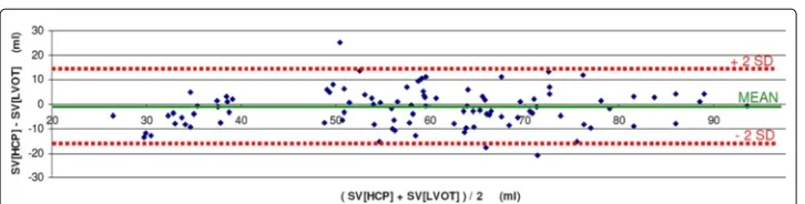
The combined results of all 7 volunteers are rendered in Figure 6 (Linear Regression) and Figure 7 (Bland Altman plot).

The Pearson correlation coefficient in Figure 6 wasR=0.892.

In the Bland-Altman plot, the mean bias was -1.6 ml, with 2SD = 14.8 ml. The upper limit of agreement was 13.2 ml, and the lower limit of agreement was -16.4 ml.

Discussion

Ex-vivo post-mortem measurements

The ex-vivo post-mortem measurements show that the spatial 2D distribution of volt-age changes over the frontal thoracic skin due to ventricular emptying (the ventricular “fingerprint”) is clearly different from the atrial “fingerprint”.

Figure 4 Typical examples of a ventricular volume-time curves (red, thick line), produced by the HCP. These volume-time curves were measured on human volunteers, in a standing position,beforeinflation of the G-suit. The vertical axis shows the ventricular volume change (V(τ )₋V(0)) in ml, as calculated using eq. 12; the horizontal axis shows the timeτ(i.e., the time that has lapsed since the last R-peak of the ECG), in milliseconds.a:volunteer with a heart rate of 69 bpm, stroke volume of 73 ml, and cardiac output of 5.0 l/min. b:volunteer with a higher heart rate of 94 bpm, stroke volume of 50 ml, and cardiac output of 4.7 l/min. In both (a) and (b), the ECG (thin line, blue) was measured simultaneously by the HCP, and has been plotted above the corresponding volume-time plot. For each of the volunteers, five different phases of the cardiac cycle (indicated byAtoFin the volume-time graphs) can be recognized:A= Isovolumetric contraction phase, B= Ejection phase,C= Isovolumetric relaxation phase,D= Rapid filling phase,E= Diastasis,F= Atrial kick. For each volume-time plot, the dashed vertical lines indicate the boundaries between the various heart phases.

about -0.03) centered around (-30,-70) is visible, as well as a positive counterpart (pur-ple, positive blob, maximum value of about 0.03) near (30, -180). In the Appendix, and more particularly in Figure 8, it was predicted that the normalized voltage change distri-bution on the thoracic skin (fingerprint) in the post-mortem ex-vivo experiments should have approximately the same appearance as if the heart were replaced by a set of elec-tric dipoles. The presence of the yellow (negative) blob and the purple, positive blob in the atrial plot in Figure 3 are in accordance with a “dipole-like field” from a set of dipoles located inside the heart.

Figure 5 Example of a plot of the stroke volume as function of time (in minutes), according to the HCP (red, continuous line), and LVot Doppler, during the G-suit experiment.The three thick dashed vertical black lines denote the following instances (from left to right, respectively): (i) starting of the inflation pump connected to the G-suit, (ii) maximum pressure reached, (iii) opening of the valve that releases the pressurized air from the G-suit immediately. During inflation of the G-suit, the stroke volume increases. Furthermore, directly after the sudden deflation at 4 minutes and 40 seconds, the stroke volume decreases. This is consistent with data from the literature (e.g. [19]).

Figure 6 Results of the G-suit validation experiments on 7 volunteers: plot of the Stroke Volume according to the HCP as function the Stroke Volume according to the LVot Doppler.Both axes are in ml. The Pearson correlation coefficient was_R=0.892. Four different marker symbols have been used to indicate the points, in which each symbol corresponds to one of the four stages during the G-suit protocol: Black diamonds = baseline, Brown triangles = inflation, Green squares = inflated, Blue Circles = deflated).

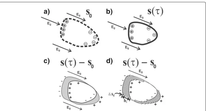
Figure 8 Schematics illustrating the relation between a volume change of some blood filled lumen (such as e.g. a ventricle) and the sum of dipoles that represent the first order alteration of the E-field due to the volume change, as explained in the first subsection of the Appendix.a:The initial volume of blood (atτ=0) is bounded by a closed surfaceA₀(indicated by the dashed line) that has non-zero values of s_{0. At each surface element}δA_{iof the surface}A₀, there is a chargeqithat is proportional to(E0·δAi). The charges on the boundary surfaceA₀are indicated by the⊕and⊖signs. (Evidently, in an applied AC current field, the boundary charges change signs continuously, along with the direction of the arrow of the appliedE_{0, with the same frequencyfof the AC current. In this schematic however, only the moments in} time are depicted in which the arrows point in one specific direction).b:Situation at some timeτ >0 during the same cardiac cycle. The volume of blood has become smaller, and is now bounded by the non-zero values ofs(τ ).c:Subtraction of the volumes from (a) and (b), in which the volume differenceV(τ )−V(0)is indicated by the grey shade. If the voltage distributions on the thoracic skin in situation (a) and (b) are denoted by(x_{, 0})and(x_,τ ), respectively, then the voltage change(x_,τ )−(x_{, 0})corresponds to s(x_,τ )−s₀(x), and hence also corresponds to the dipoles in (b) minus the dipoles in (a).d:The grey-shaded volume differenceV(τ )−V(0)equals the sum of a set of small rectangular beams :

V(τ )−V(0) = _ih_i·(δA_i), which is quite similar to the sum of the dipoles formed by the charges at the end-points of the rectangular beams, corresponding to the dipole interpretation of the charges in (c).

thoracic skin. Therefore, only the upper part of the top blob (orange, negative) was located on the post-mortem thorax in the ex-vivo ventricular fingerprint measurements, at about (30,-180) in the left panel in Figure 3.

In-vivo tests on human volunteers

The shapes of the ventricular volume-time curves (see Figure 4) were consistent with the time curves from the literature. The realistic shapes of the ventricular volume-time curves produced by the HCP during the tests on human volunteers indicate that the atrial and ventricular fingerprints are indeed different enough to enable the HCP algorithm.

One volunteer (volunteer♯8) was excluded from the validation section because LVot Doppler incidently detected a leakage of the mitral valve. Interestingly, the HCP has produced a volume-time curve for this volunteer that is distinctly different from the volume-time curves of the other volunteers, and, moreover, this particular volume-time curve was assessed by cardiologists to be typical for mitral valve leakage. Further research is warranted to investigate if the HCP not only can produce reliable stroke volume val-ues, but also may be used to determine particular patterns in the volume-time curves to diagnose e.g. diastolic dysfunction, cardiomyopathy or valvular disease.

Therefore, the ventricular volume-time curves have the potential of being a useful diagnostic monitoring tool as well.

Comparison of the VFR with other techniques

In contrast to Impedance Cardiography (ICG), the VFR method uses multiple electrodes to create input for 6 independent and simultaneous voltage input channels. Our method isnotbased on impedance cardiography (ICG) algorithms, since we do not calculate any impedance measure, but use spatial patterns to retrieve volume changes of specifically the ventricles.

Some ICG-like techniques (such as e.g. Woltjer et al [20]) use multiple electrodes, but - in contrast to our method - still measure only one single voltage, because the leads of many of these electrodes are interconnected to form a single input channel.

Comparison of the bias and precision (2SD) of the prototype of the HCP in this study with that of other techniques as listed in e.g. [3], shows that the HCP yielded satisfactory results as a completely non-invasive technique.

Sources of inaccuracy

There are three principal factors that may affect the validity of the relation in eq.(7): (i) A mismatch (in thecranial-caudaland theleft-rightdirections) between the theo-retical optimal electrode positions with respect to the volunteers’ heart, corresponding to the ex-vivo calibration measurements, and the actual electrode positions that result from placing the electrodes on basis of externally visible anatomical landmarks (viz. the incisura jugularis) on a volunteer. Since considerable anatomical differences exist between the various volunteers (i.e. for each volunteer the position of the heart with respect to the incisura jugularis may be different because of a different inclination angle of the heart axis or vertical position of the heart), we have installed into our experimental HCP set-up a piece of software that prevents this mismatch by performing simulated “virtual displace-ments” of the heart of the ex-vivo experiments within the algorithm, in order to find an optimal match between the measuredv_{meas(τ )and key features from the fingerprints}

during a brief initial calibration phase; subsequently the fingerprint vectorsf_Aandf_V are adapted accordingly, and theW_AandW_Bvectors are calculated that are used from that moment onwards for that specific volunteer.

(ii) A mismatch between the distance from the skin to the heart (in thefrontal-dorsal

volunteer, which however should relate to the same ventricular volume change. Therefore, the correct ventricular volume changeV(τ )−V(0)should be calculated as

V_{(τ )−}V₍₀₎₌Kvolunteerψ (τ )Vcalib

in whichK_{volunteeris a constant scaling factor that may be different for each volunteer. This} scaling factor has been assessed by an initial calibration procedure at the beginning of the actual HCP measurements for each volunteer, using Doppler Ultrasound (see section Methods: in-vivo tests of the HCP on volunteers for details). In the future, a stand-alone initial calibration procedure to measureKvolunteer, without the need for Doppler Ultra-sound, may be incorporated into the HCP system, using an extra measurement invoking the Principle of Reciprocity: In this auto-calibration procedure, the measuring electrodes are used temporarily for current injection. In an ex-vivo study and in computer models, we have shown that, invoking the reciprocity theorem of electromagnetic fields, this pro-cedure is capable of assessing the attenuation of signals between the heart and the skin, thus making an initial calibration using LVot Doppler unnecessary.

(iii) Errors due to the assumption of linearity in eq.(7) itself. This is a major point that deserves closer investigation. As has been indicated above, any calculation of volt-age changes on basis of volume changes of blood-filled lumina such as the ventricles, is a non-linear problem, and therefore the magnitude of the inaccuracy that results from the linear assumption in eq.(7) needs to be assessed. Therefore, in the Appendix section, the (non-linear) relation between volume change and the measured data is investigated.

In the appendix, in Figure 9, three major sources of non-linearity are depicted schemat-ically. Using the formula (eq.(34)) derived in the appendix, confines to the maximal deviations from linearity have been calculated, yielding the graphs rendered in Figure 10. For a volume change that equals two times the calibrated initial volume change, the non-linear effects may cause a voltage change that is maximally 14% higher than the linear approximation. Using the linear approximation therefore leads to anoverestimationof the stroke volume of maximally 14% in this case.

For a volume change that equals half of the calibrated initial volume change, the non-linear effects may cause a voltage change that is maximally 6% lower than the non-linear approximation. In this case, the linear approximation therefore leads to an underestima-tion_{of the stroke volume of maximally 6%.}

Conclusions

A new non-invasive, operator-free, continuous ventricular stroke volume monitoring device (HCP) has been developed in our group, producing the average stroke volume (SV) for each period of 20 seconds, as well as ventricular volume-time curves for each cardiac cycle. A preliminary validation study on 7 human volunteers, using LVot Doppler as a reference technique, yielded a good correlation (Pearson correlation coefficient R=0.892) between the stroke volume according to HCP, and the stroke volume according to LVot Doppler.

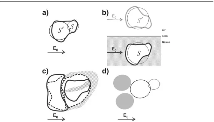
Figure 9 Schematics representing various anatomical and cardiological features that contribute to the non-linearity in the relation between voltage change and volume change.a:The non-spherical shape of the ventricles (feature (a) in the appendix) corresponds to an assembly of multiple spheres. In this figure, a simple representation of a ventricle, using only two spheres (indicated bySandS′_{), is depicted.}

During ventricular systole, the volume of each sphere decreases. The voltage increase, due to the volume decrease of the combination of the two spheres in close proximity, is less than the sum of the effects would have been when the effects of both spheres would have been calculated separately, without taking into account the close proximity of the two spheres. For instance, if the volume change ofS′_{increases (i.e.,}S′

becomes extra small near the end of the ventricular systole), then the strength of the incident field onS

decreases during ventricular systole, thus diminishing the effect of the decrease of the volume ofSon the

measured voltage. Therefore, the non-linearity due to this “shadow effect” ofS′_onS(and vice versa) yields a negativeηvalue, viz.η= −0.033.b:The proximity of the heart to a boundary surface (skin-air), viz. the frontal surface of the thoracic skin. The non-linear effect due to the proximity to this boundary surface has been

calculated using the Method of Image Charges [21], resulting inη=0.035. A decrease ofSwould entail a

decrease of the mirror sphereS′_{as well. A decrease of the volume of}S′_{would cause an increase of the}

strength of the incident field onS, thus increasing the effect that the decrease ofSwould have on the

measured voltage. Hence the value ofηis positive in this case.c:The cardiological phenomenon that a

decrease of ventricular volume is generally accompanied by a simultaneous increase in atrial volume, and vice versa. In this schematic, the continuous lines represent the end-systolic situation, whereas the dotted lines refer to the end of the diastole.d:The same as inc, but now depicted using spheres, yieldingη=0.107.

The combined effect of the phenomena depicted inbandcyields a “worst case” ofη=0.142. The “atrial”

spheres are depicted in opaque grey.

The shapes of the ventricular volume-time curves (see Figure 4) were realistic, and consistent with the volume-time curves from the literature. Therefore, the ventricu-lar volume-time curves have the potential of being a useful diagnostic monitoring tool as well.

Appendix

In this appendix, the necessary theoretical underpinning of the fundamental equation 7, which constitutes the basis of the VFR method, is provided.

A1: fundamental relation between measured voltages and volume changes

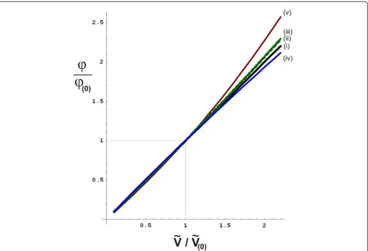
Figure 10 Graphs indicating boundaries to the theoretically possible deviations from a linear relationship between relative volume change and relative voltage change (as indicated in assumptionL,eq.(16)), for various basic anatomical and cardiological features as listed in the appendix.In all graphs, the theoretical ratioϕ/ϕ(0)(vertical axis, dimensionless number) has been calculated

as function of the ratioV/V(0)(horizontal axis, dimensionless number), in whichϕ(0)is the given initial

voltage change resulting from the known volume changeV(0)as measured by the initial calibration

procedure duringn=0. In the ideal (and unrealistic) case that assumptionLwould hold exactly, the relation ϕ/ϕ(0)=V/V(0)would hold exactly as well, as represented by the identity line (thick continuous black line,

indicated by(i)). Thedotted green line, indicated by(ii), is a graph of eq. (34) withη=0.035, which is a second order calculation of the maximum deviation from linearity due to the presence of a boundary plane (representing the frontal surface between the conducting thorax and the insulating air) in the form of the frontal thoracic skin (feature (b) in the appendix, as depicted in Figure 9b), using the method of image charges [21]. The slender area between this dotted green line and the identity line (black solid line) represents the area containing all possible deviations from linearity (i.e., the solid black line) due to feature (b). Similarly, a graph was calculated for feature (b) using the entire perturbation series in eq.(31), resulting in thecontinuous green line, (iii). Furthermore, thecontinuous blue line (iv)represents the maximum deviation from linearity due to the non-spherical shape of the ventricles (feature (a)), using the entire perturbation series withη= −0.033. Finally, the maximum deviation from linearity due to the fact that (generally) the atria are filling up when the ventricles are emptying and vice versa (feature (c)), in combination with feature (b), results in thecontinuous red line (v), using the entire perturbation series andη=0.142.

Furthermore, we concentrate on the stroke volume of each heart beat, and enumerate the heart beats using an index(n)(n ∈ {1, 2, 3,. . .}), and define V₍n₎as the stroke volume

of beat numbern. Letvmeas_,(n₎be defined as thevmeasvector at the moment in time of

maximum volume change during cardiac cycle numbern(i.e., the end-systolic moment in

cardiac cycle numbern_{), and let the index (0) refer to the first heartbeat after the start of} the measurements (baseline condition,n=0). Evidently, in the course of time aftern=0, during later heartbeats, the stroke value may differ from the initial stroke valueV₍₀₎

In order to evaluate the limitations to the assumed linearity in eq.(7), it is examined to what extent the following “assumption of linearity”L_{is valid:}

in whichλ(n) is a scalar (representing the proportionality factor for cardiac cycle

num-bern), and in which the 6 valuesϕ(_meask) (k ∈ {1, 2,. . ., 6}) inv_measare caused by volume changes in the only volumes present, i.e. the ventricles. The assumptionLthus reads that if during cardiac cycle # (n) the stroke volumeV(n)equalsλ(n)times the initial stroke

vol-umeV(0), then all 6 voltages invmeas,(n)would equalλ(n)times the initial voltages during

cardiac cycle # (0) as well.

Evidently, based on the general fact that calculation of voltages from conductivity dis-tributions is a non-linear problem, it is clear on beforehand that the assumptionL_will

not be true with exact precision; hence the≈-sign in eq.(16)

In the experiments on human volunteers, an initial calibration procedure using Doppler Ultrasound has been performed at the start of the experiment, and hence the value of the actual initialV(0)has been provided by Doppler Ultrasound for each volunteer.

The assumptionLcan only be valid (approximately) if, for any value ofn>0, the shape change of the volume, during the volume change during cardiac cycle numbern, is not completely deviant from the shape change of the volume duringn=0. In other words, we make the assumption that sudden ruptures or other sudden abnormal patterns of volume changes are excluded. We will refer to this assumption as the “assumption of regularity

R”, and will specify this assumptionRmore precisely later on in this subsection.

In order to assess the limits of accuracy of the assumptionL, a fundamental relation between the measured relative voltage changesϕ and volume changes of blood-filled lumina is derived below, starting with explaining the nature of the applied current field.

The oscillation frequencyf of the measured AC voltages, which equals the oscillation frequency of the current injected into the patient via the current feeding electrodes on the legs and arms or head, is high in comparison to the physiological processes like respiration or the motion of the heart during the cardiac cycle. Furthermore, the frequencyf is low enough to let the values of 2πfǫ (in whichǫis the dielectric permittivity) be negligible with respect to the differences in specific conductivityσ for the relevant tissues [22]. Therefore only the amplitude of the measured AC voltages needs to be considered; in our set-up each(meask) (τ )value was defined as theamplitude of the oscillating voltage measured between the electrodesekandek−1at timeτ. This amplitude of the voltage was established every 5 milliseconds.

Directly below, a relation between the measured voltage changesϕand volume changes of blood-filled lumina is derived, on basis of the law of conservation of charge (the continuity equation) and Ohm’s law.

Since the current sources are applied to the head or arms and legs, there are no current injection electrodes present on the thorax. Therefore, the continuity equation for points inside the thorax reads:

∇ ·J(x)= 0 for allx∈T (17)

in whichxis a three-dimensional spatial coordinate ( i.e.xdenotes a point within 3D space), and J(x) denotes the current density at pointx, and T denotes the complete thorax, including the thoracic skin, and everything inside the thorax.

Substituting Ohms lawJ = σEin eq. (17), in whichσ denotes the conductivity andE

denotes the electric field, and applying the general mathematical identity

we may rewrite eq. (17) as

σ∇ ·E₊ E_{· ∇σ =0 (18)}

Using _σ1∇σ = ∇logσ, this can be written as

∇ ·E_{= −}E_{· ∇logσ (19)}

Let the 3D vector field−∇log(σ (x_{))be denoted as}s₍x_). Therefore we now have:

∇ ·E₍x₎₌E₍x_{) ·}s₍x_{) (20)}

This is an implicit equation forE₍x_{)for a given}s₍x_{)distribution. For a model of the} human anatomy in which a limited number of tissue types are defined (such as “blood”, “muscle tissue”, “bone”, etc.), the spatial conductivity distributionσ (x_{)is piecewise}

con-stant; i.e. the value of s₍x_{) is zero everywhere, except at the boundary between two}

different tissue types. For a sharp boundary, we have [21]:s₍x₎₌₂n_ˆσ1−σ2

σ1+σ2, in which ˆ

n_is

the normal unit vector perpendicular to the boundary surface at pointx_{, andσ1andσ2} are the specific conductivities of the two tissue types that meet at the boundary surface.

Since∇ ·E ₌ ρ

ǫ (according to the Maxwell equations, in whichρis the charge

den-sity andǫis the dielectric constant), the right-hand side of eq.(20), i.e.E₍x_{) ·} s₍x_{), may} be regarded as a charge density divided by the dielectric permittivityǫ. Therefore, points within the thorax having non-zero values ofs₍x_{)may be considered as equivalent} “sec-ondary” sources, responsible for non-zero divergence ofE_{within the thorax at points on} boundary surfaces. The effect of these secondary sources on the rest of the thorax (includ-ing the measur(includ-ing electrodes on the thoracic skin) may be calculated us(includ-ing the Green

functionGof the Poisson equation.

In order to use this for the particular case of ventricular volume changes, consider eq.(20) at two instances in time:

∇ ·E₀₍x₎₌E₀₍x_{) ·} s₀₍x_{)at timeτ =0, i.e. at the time of the R-peak of the ECG, and}

∇ ·E₍x_{,τ )=}E₍x_{,τ )·} s₍x_{,τ )at some later instant during the same cardiac cycle (τ =0).} Subtracting the equation forτ =0 from the equation forτ =0, and using the extra sym-bolsE_ands_withE₍x_{,τ )=} E₍x_{,τ )−}E₀₍x_)ands₍x_{,τ )=} s₍x_{,τ )−}s₀₍x_{)to indicate the} difference fields, yields

∇ ·E₍x_{,τ )=}E₀₍x_)·s₍x_{,τ )}

(⋆)

+E₍x_{,τ )·}s₍x_{,τ )}

(⋆⋆)

(21)

This is still an implicit equation from whichE_{can not be calculated directly.}

In eq.(21), the first term (E₀₍x_{) ·}s₍x_{,τ )), indicated by (⋆), represents the first order} approximation, whereasE₍x_{,τ )·}s₍x_{,τ ), indicated by (⋆⋆), represents the self-reference in} this equation, which leads to higher-order corrections in the form of a perturbation series if an exact expression forE_{is derived. In the appendix, the exact solution to eq.(21) is} presented in the form of such a perturbation series.

Using the first order approximation of eq.(21), i.e.∇ ·E(τ )₌E0 ·s(τ ), the expression forE(x,τ )reads:

E(x,τ )_{= ∇}[G∗ (s(ξ,τ)_·E0(ξ))] (22)

in which∗denotes the 3D spatial convolution, andξ denotes points in 3D space over which the convolution takes place, and G denotes the Green function of the Poisson equation (G(x₋ξ)=1/(4π(x₋ξ)·(x₋ξ))). Hence the change in the voltage differ-ence(k)between two electrodesek andek₋1(at positionsxk andxk−1on the skin) as function of the timeτ during one single heartbeat is calculated as:

(k)(τ )−(k)(0)=

thorax

d3ξG(xk−1−ξ)−G(xk−ξ)s(ξ,τ )·E0(ξ) (23)

in which_thoraxd3ξdenotes integration over 3D space. withξdenoting points in 3D space. From this equation, a basic relation between voltage changes and volume changes can be derived, as is indicated in Figure 8.

Consider, as a simplified example, the boundary of a single volume of blood within an environment of tissue. This boundary is rendered in Figure 8a for the initial situation at

τ ₌ 0. The value ofs(x, 0)is zero everywhere, except at the boundary. At a later instant

τESduring the same cardiac cycle (in which the subscript “ES” refers to “end-systole”), the volume of blood has reached its maximum volume change.

As is explained in the legend of Figure 8, the subtraction of Figure 8a from Figure 8b yields Figure 8c, in which the equivalent charge distributionss·E0(x)are rendered that give rise to(k)(τES)−(k)(0)in eq.(23). All situations rendered in Figure 8 are from one single heartbeat, i.e. cardiac cycle numbern. The relation with maximum volume change (i.e., the stroke volumeV(n)of cardiac cycle numbern) is now indicated in Figure 8d. The

volume changeV(n) =V(τES)−V0, in whichV(τES)relates to Figure 8b, andV0relates to Figure 8a, can be calculated as the sum of the set of small grey rectangular beams in Figure 8d. Let the small grey beams be enumerated using the indexi. Since the direction of the small grey beams, and hence ofδAi, may be chosen freely when calculating a volume, we chooseδAito be parallel toe0, in whiche0is the direction parallel toE0, with

E0=E0e0andδAi=Aie0andhi=hie0

Therefore the volume change now reads

V(n)=V(τES)−V(0)=

i

hi·(δAi)=

i

hiAi (24)

The model depicted in Figure 8 can incorporate volume changes in a direction perpen-dicular toe0as well: If the volume is becoming smaller in a direction perpendicular toe0, then some rods near the boundary become gradually shorter until they vanish completely (when the length of the rod becomes zero). If the volume is becoming larger in a direction perpendicular toe₀, some vanished rods with length zero obtain non-zero length again (effectively adding new rods at the boundary of the volume).

Similarly, the chargess·E0(x)may be considered to be a set of dipolespi =qihie0(as explained in Figure 8), enumerated by the indexi, with dipole lengthhiand chargeqi.

At this point, we provide a more precise definition of the “assumptionR_{” (the}

assump-tion of regularity in the volume changes) that has been menassump-tioned at the beginning of this subsection:

assumptionR_{: ifV(n)}=λ(n)V(0), then∀i:hi,(n)=λ(n)hi,(0) (25)

With this assumptionR_{, and the dipole modeling described above, the voltage change}

k(τES)−k(0)in eq.(23) for cardiac cycle #nmay be written as:

σtissue)[21] in the simple example of Figure 8, this yields :

k_(n)(τES)−k_(n)(0)=

from which it becomes apparent that, having used the assumption of regularityR_(eq.

(25)) and the first order approximation in eq.(22),k_(n)(τES)−k₍n)(0)is indeed

propor-tional toλ(n)ihi,(0)Ai, and hence assumptionLholds in this case. Furthermore, eq.(27)

shows thatk_(n)(τES)−₍k_n)(0)is proportional to the incident field strengthE0as well.

As has been indicated before however, it is clear on beforehand that the assumptionL

will not be true with exact precision, due to the fact that the relation between volumes and voltages in fundamentally non-linear. The strength of the non-linear effects will be examined in the next subsection (A2).

A2: non-linear effects

In the subsection above, the first order explicit equation (22) has been derived from the general implicit equation (21), by neglecting the self-referential term indicated by(⋆⋆)

in eq.(21). The exact version of equation (22) however, i.e. without neglecting the self-referential term indicated by(⋆⋆)in eq.(21), reads:

E(x)= ∇

thorax

d3ξG(x−ξ)E₀(ξ)·s(ξ)+s(ξ)·E(ξ) (28)

and hence the voltage difference between the two electrodesekandek−1equals:

(k)(τ )−(k)(0)=

thorax

d3ξG(x_k−1−ξ)−G(x_k−ξ) E₀(ξ)·s(ξ)+s(ξ)·E(ξ)

(29)

In order to transform equation (28) into an explicit equation forE_{(and hence solving} eq.(29) as well), an iterative substitution method is used that is comparable to the itera-tive substitution that produces the Born-Neumann series from the Lippmann-Schwinger equation, i.e.: the symbolEappearing in the right-hand side of eq.(28) is replaced by the expression that is formed by the entire right-hand side of eq.(28). This results in a

equation, and hence the substitution procedure can be repeated, which yields an iterative substitution procedure.

In the top line of eq.(30) the result of the iterative substitution is rendered, and sub-sequently “expanded” by distribution through parentheses (in the second line of eq.(30)), yielding a perturbation series:

in which, again, the symbol∗denotes the convolution operator in three dimensions. The voltage difference between the two electrodesekandek−1hence reads:

(k)(τ )−(k)(0)=

An important parameter for the assessment of convergence of the seriesA_{in eq. (30)} and eq.(31)) is the fraction_|E|E(x)|

0(x)|.

If the fraction_||EE₀₍(xx)|_)| is small compared to one, then the higher order (largeϑ) terms in (31) become rapidly irrelevant with increasingϑ.

Since the cardiac motion causes only a small distortion of the applied current field, we have that_|E|E(x)|

0(x)| is indeed small compared to one, as can be shown for the theoretical case of a single spherical volume representing a ventricle in a homogeneous surroundings. For this theoretical case, the maximum value of _|E|E(x)|

0(x)| outside the sphere can be calculated exactly, and equals 0.14 for the conductivity values of blood and muscle tissue, and is reached near the surface of the sphere on the central axis of the sphere parallel to the incident fieldE_{0. For most other positions}x_{, the value of} |E(x)|

|E₀(x)| is much lower.

We now use eq.(31) to examine the non-linear character of the relation between vol-ume changes and the measured(k₎

(τ ) − (k₎

(0)by adding various anatomical and cardiological features, starting with the above mentioned simple theoretical case of a sin-gle spherical volume of blood (withσblood) inside an infinite homogenous surroundings (with specific conductivityσtissue). From the literature [21] it is known that, in this spe-cific case, the electric field in the surroundings of the sphere is exactly equal to the sum of the incident field plus the field from a single dipole located at the center of the sphere. As a result, the(k)(τ ) − (k)(0)will be exactly proportional to the volume of the sphere.