USING LABEL NOISE ROBUST LOGISTIC REGRESSION FOR AUTOMATED
UPDATING OF TOPOGRAPHIC GEOSPATIAL DATABASES
A. Maas *, F. Rottensteiner, C. Heipke
Institute of Photogrammetry and GeoInformation, Leibniz Universität Hannover - Germany (maas, rottensteiner, heipke)@ipi.uni-hannover.de
Commission VII, WG VII/5
KEY WORDS: Change detection, label noise, logistic regression, supervised classification
ABSTRACT:
Supervised classification of remotely sensed images is a classical method to update topographic geospatial databases. The task requires training data in the form of image data with known class labels, whose generation is time-consuming. To avoid this problem one can use the labels from the outdated database for training. As some of these labels may be wrong due to changes in land cover, one has to use training techniques that can cope with wrong class labels in the training data. In this paper we adapt a label noise tolerant training technique to the problem of database updating. No labelled data other than the existing database are necessary. The resulting label image and transition matrix between the labels can help to update the database and to detect changes between the two time epochs. Our experiments are based on different test areas, using real images with simulated existing databases. Our results show that this method can indeed detect changes that would remain undetected if label noise were not considered in training.
*
Corresponding author
1. INTRODUCTION
Topographical databases are very important for applications such as navigation or city planning. Keeping such a database up-to-date manually has been estimated to require up to 40% of the costs for the original data acquisition (Champion, 2007), which indicates that this process should be automated. In this context, the primary data source most frequently used is remotely sensed imagery. If the sensor data used for the original data acquisition are not available, a typical work flow for automated updating of topographic databases starts with the classification of the new sensor data. In a second step, the classification results are compared with the database in order to detect areas of change e.g. (Vosselman et al., 2004). Based on the detected changes, the database can then be updated. For the first step, supervised classification algorithms are frequently used because they are more easily transferred from one data set to another one. The reason for this is that supervised methods rely on representative training data to train the underlying classifier, thus adapting it to changes in the appearance of the objects.
This flexibility comes at the cost that training data, consisting of image subsets with known object labels, have to be generated in advance, typically in a time-consuming and costly manual process. Thus, it would be desirable to reduce the amount of training data required. One strategy to achieve this aim is to use the existing database to provide the necessary class labels. Such a procedure has to take into account that the database may be outdated, so that some of the class labels derived from the original map might be wrong. However, in general changes will only affect a relatively small part of a scene, so that one can assume the majority of the class labels to be correct.
In this paper we propose a new supervised classification method that uses existing database information for training. Unlike most of the existing work in this context, we do not just eliminate
training samples having a wrong label as outliers, but we resort to a training method that is tolerant to these errors. In particular, we use a label noise tolerant version of logistic regression (Bootkrajang & Kabán, 2012), a probabilistic method that does not only reduce the impact of label noise in the training process, but also delivers an estimate about the amount of change in a scene. After applying the resultant classifier to the new sensor data, we can compare the classification results to the original database and, thus, obtain change in land cover. No manually labelled training data are required. Our method is evaluated using several data sets with different degrees of simulated changes to show the benefits, but also the limitations of the proposed method.
2. RELATED WORK
affected by gross errors called label noise, which has to be considered in the training process.
Training under label noise is a well-studied problem, for example in fields such as epidemiology, econometrics and computer-aided diagnoses. Frénay and Verleysen (2014) differentiate three types of statistical models for label noise. The noisy completely at random (NCAR) model assumes the occurrence of a label error to be independent from all other variables, including the class label. It is characterized by a single parameter, namely the probability of an error. In the noisy at random (NAR) model, the probability of an error depends on the class labels, so that it is parameterized by a square transition matrix whose elements describe the probability for a specific type of error affecting two classes. The most complex model is called noisy not at random model and additionally considers dependencies between labelling errors and the observed data.
According to Frénay and Verleysen (2014), there are three strategies for dealing with label noise. The first one is to use a classifier that is robust to label noise by design, e.g. random forests. However, such methods still have problems with a large amount of label noise. The second strategy tries to identify the incorrect training samples in order to remove them from the training set before the actual training procedure. The authors state that such data cleansing approaches tend to eliminate too many instances, which may lead to a decreased classification performance. Finally, the third strategy consists of learning algorithms that are tolerant to noisy training data. In this context probabilistic approaches can be distinguished from non-probabilistic ones. Probabilistic models learn the parameters of a noise model, e.g. the elements of the transition matrix for the NAR model, jointly with the parameters of a classifier that would best separate the data based on the (unknown) true labels of the training samples. This strategy is followed by Bootkrajang and Kabán (2012), using logistic regression as a base classifier. Li et al. (2007) achieve a similar result on the bases of a kernel Fisher discriminant. Bootkrajang and Kabán (2012) report results for the classification of entire images with the purpose of image revival, but not for a classification on a pixel level. Non-probabilistic methods focus on making non-probabilistic classifiers such as support vector machines (SVM) tolerant to label noise (An & Liang, 2013), but typically do not estimate the parameters of a noise model.
To the knowledge of the authors most existing approaches for considering label noise in remote sensing are based on data cleansing. For instance, Radoux et al. (2014), deriving training data from an existing map, present two techniques for eliminating outliers. The first one removes training samples near the boundaries of land cover types, whereas the other one assumes a Gaussian distribution of spectral signatures and removes outliers based on a statistical test. These methods seem to be tailored to data of low ground sampling distance (300m). It is doubtful whether the model assumptions can be transferred to high resolution data, where each class may correspond to multiple clusters in feature space. A similar method was used for map updating in (Radoux & Defourny, 2010), using Kernel density estimation for deriving probability densities. The error rates in the original data were relatively low. Jia et al. (2014) use all pixels from an existing map for training and eliminate samples that receive another class than the one indicated in the original data. Büschenfeld (2013) uses land cover data from a geographical information system (GIS) for generating training samples. He iteratively applies SVM, eliminating training samples that are assigned to another class than indicated by the
observed label or that show a high uncertainty. The entities to be classified are land cover objects from the GIS.
Mnih and Hinton (2012) are among the few authors using maps for label noise tolerant training. Their method is based on deep learning, but they only present a solution for a binary classification problem. Bruzzone and Persello (2009) propose a context-sensitive semi-supervised SVM, which is supposed to be robust to label noise. This improvement is realized by inclu-ding information of the pixels in the neighbourhood of the training samples in the learning process. However, no probabi-listic label noise model is used. The authors claim that such a strategy allows the use of existing maps for training, but this topic is not elaborated further.
This paper presents a new method for change detection between an outdated database and current remotely sensed images without using manually labelled training data, just relying on the database. Unlike most existing work, we apply label noise tolerant classification to cope with incorrect training labels. In particular, we apply label noise tolerant logistic regression (Bootkrajang & Kabán, 2012), a probabilistic method that also provides estimates for the parameters of a NAR model which can be interpreted as probabilities for specific types of change. In order to consider local context, we integrate this classifier in a Conditional Random Field (CRF) model. The resulting label image is compared with the database to detect changes. We evaluate our method for different degrees of label noise and compare the results to those achieved by random forests.
3. LABEL NOISE TOLERANT CHANGE DETECTION
3.1 General Idea
For our task we assume the existing database and the image data to be available in raster format, defined on the same grid. The data consist of N pixels, each pixel represented by a feature vector of dimension F. The existing database contains an observed class label for each pixel n, where denotes the set of classes and K is the total number of classes. As the database may be outdated, the observed label may differ from the unknown current label
of that pixel that corresponds to the updated database information and has to be estimated from the data. Changes are determined implicitly as pixels where the observed label differs from the current one ( ).
3.2 Label Noise Tolerant Logistic Regression
Multiclass logistic regression is a probabilistic discriminative classifier that directly models the posterior probability p(Cn|xn)
of a class label Cn given the feature vector xn. A feature space
transformation (xn) is applied to achieve non-linear decision
boundaries in the original feature space. That is, rather than to xn, the classification is applied to a vector (xn) which has a
higher dimension than xn and whose components may be
arbitrary functions of xn. For instance, one can use quadratic
expansion, i.e. (xn) contains the original features as well as all
squares and mixed products of features. In addition, (xn)
contains a bias feature that is assumed to be a constant with value 1 without loss of generality. The model of the posterior is based on the softmax function (Bishop, 2006):
(1)
where wk is a vector of weight coefficients for a particular class
Ck that is related to the parameters of the separating hyperplanes in the transformed feature space. As the sum of the posterior over all classes has to be 1, these weight vectors are not independent. This fact is considered by setting w1 to 0. The
remaining weights are collected in a joint parameter vector
w=(w2
T, …
wK
T
)T to be determined from training data.
It is our goal to train a classifier that directly delivers the current labels Cn. However, our training data consist of N independent
pairs (xn, ) of a feature vector and the corresponding
observed class label from the existing database. In order to determine the most probable values of w, we have to optimise the posterior of w given the training data (Bishop, 2006):
(2)
In the presence of label noise, the observed label is not necessarily the label which should be determined by maximising the posterior in eq. 1. Bootkrajang and Kabán (2012) propose to determine the probability required for training as the marginal distribution of the observed labels over all possible states of the unknown current labels Cn. This leads to (Bootkrajang & Kabán, 2012):
(3)
or where we introduced the short-hands
, and
.
In eq. 3 is identical to the posterior for the unknown current label Cn, modelled according to eq. 1. The
probabilities are the parameters of the NAR model according to (Frénay & Verleysen, 2014), describing how probable it is to observe label if the true label indicated by the feature vector is From the point of view of change detection, these probabilities are closely related to the probability of a change from class to , though the direction of change according to the definition in eq. 3 is actually inverted. If we differentiate K classes, there are, consequently, K x K such transition probabilities, which we can collect in a K x K transition matrix with (a,k) = ak.
We use a Gaussian prior with zero mean and isotropic covariance · I, where I is a unit matrix, for the regularisation term p(w) in eq. 2. Finding the maximum of eq. 2 is equivalent
to finding the minimum of the negative logarithm, thus of
. Plugging eq. 3 into eq. 2 and taking the negative logarithm yields
, (4)
where is an indicator variable taking the value 1 if and 0 otherwise. As is nonlinear, minimisation has to be carried out iteratively. Starting from initial values w0, we apply gradient descent, estimating the parameter vector w in iteration using the Newton-Raphson method (Bishop, 2006):
, (5)
where is the gradient vector and H is the Hessian matrix. The gradient is the concatenation of all derivatives by the class-specific parameter vectors wj, with (Bootkrajang & Kabán, 2012)
(6)
where
. The Hessian Matrix consists
of (K - 1) x (K - 1) blocks with (Bootkrajang & Kabán, 2012)
, (7)
where I is a unit matrix with elements Iij, (·) is the Kronecker
delta function delivering a value of 1 if the argument is true and 0 otherwise, and
. (8)
Optimising for the unknown weights by gradient descent as just described requires knowledge about the elements of the transition matrix , i.e. the parameters of the noise model. However, these parameters are unknown. Bootkrajang and Kabán (2012) propose an iterative procedure similar to expectation maximisation (EM). Starting from initial values for , e.g. based on the assumption that there is not much change (leading to large values on the main diagonal only), the optimal weights can be determined. Using these weights, one can update the parameters of according to (Bootkrajang & Kabán, 2012)
(9)
where
.
These values for the transition matrix can be used for an improved estimation of w, and so forth. Thus, the update of w and alternate until a stopping criterion, e.g. related to the change of the parameters between two consecutive iterations, is reached. Note that the parameters w thus obtained are related to a classifier delivering the posterior for the unknown current labels Cn (eq. 1).
3.3 The Conditional Random Field (CRF)
current labels Cn introduced in Section 3.1 that correspond to
the updated database information. The edges of the graph model dependencies between the random variables corresponding to the nodes. We connect direct neighbours on the basis of a 4-neighbourhood of the image grid by edges. Rather than classifying each pixel n of an image individually based on locally observed features, the entire configuration of labels, collected in a vector C = (C1, …, CN)
T
is determined simultaneously using all the observed data x, i.e. all features observed at the individual pixels. CRF are discriminative models, so that the posterior P(C|x) for the entire classified image C given the data x is modelled directly according to (Kumar & Hebert, 2006):
(10)
In eq. 10, Z is a normalization constant which is not considered further in the classification process because we are only interested in determining the label configuration C for which P(C|x) max. The association potential A is the link between the data x and the label Cn of pixel n. A(Cn, x) may depend on
the entire input image x, which is often considered by using site-wise feature vectors xn(x) that may be functions of the
entire image. Any discriminative classifier can be used in this context; we use logistic regression, thus A(Cn, x) = ln p(Cn|xn),
where p(Cn|xn) is determined according to eq. 1. The definition
of xn = xn(x) depends on the available data.
The terms I(Cn, Cm, x) are called the interaction potentials; they
describe the context model. The sum over the interaction potentials is taken over all pairs of pixels n,m connected by an edge; thus, is the set of edges in the graph. The interaction potentials also depend the data x. We use the context-sensitive Potts model for the interaction potential, which results in a data-dependant smoothing of the resultant image (Shotton et al., 2009):
(11) Again, (·) is the Kronecker delta function, whereas the coefficients and influence the overall degree of smoothing and the impact of the data-dependant term, respectively. The parameter D is the average squared gradient of the image.
We train the association potentials independently from the interaction terms, using the method described in Section 3.2. The parameters of the interaction potentials ( and ) could be determined by a procedure such as cross-validation, but we use values found empirically. For the determination of the optimal configuration of labels given the model of the posterior we use loopy belief propagation (Frey & MacKay, 1998).
4. EXPERIMENTS
4.1 Test Data and Test Setup
We use three data sets in our experiments. The first dataset consists of a part of the Vaihingen data contained in the ISPRS 2D Labelling Challenge (Wegner et al., 2015). We use eleven of the patches provided for the test, each about 2,000 x 2,500 pixels in size. For each patch, a colour infrared true orthophoto (TOP) and a digital surface model (DSM) are made available, both with a ground sampling distance of 9 cm. Furthermore, all
the patches used in this paper belong to the training set of the labelling challenge, so that reference data are available in the same grid as the other data. The reference differentiates the six classes impervious surfaces, building, low vegetation, tree, car, and clutter/background. As cars are not considered to be contained in topographic databases, we merged this class with impervious surfaces. For each pixel, we defined a five-dimensional feature vector xn(x) consisting of values for the
normalised difference vegetation index (NDVI), the normalised digital surface model (nDSM), indicating the heights above ground, the red band of the TOP, smoothed by a Gaussian filter with =2, and hue as well as saturation obtained from the TOP, both smoothed by a Gaussian filter with =10. These features were selected from a larger pool of generic features based on the feature importance analysis of a random forest classifier (Breiman, 2001).
The other two data sets, subsets of the data used in (Hoberg et al., 2015), are based on satellite imagery. Data set 2 consists of a subset of a Landsat image of an area near Herne, Germany, covering 8.6 x 5.9 km² with a GSD of 30 m (about 350 x 300 pixels), acquired in 2010. Only the red, green and near infrared bands are available to us. The reference contains three classes, namely residential area, forest and cropland. Data set 3 consists of a RapidEye image with a GSD of 5 m of an area near Husum, Germany, also acquired in 2010. The area covered by this image is about 3.500 x 1.900 pixels or 16.8 x 9.6 km², and, again, only the red, green and near infrared bands are available to us. The reference contains the classes residential area, rural street, forest and cropland. For both data sets we selected seven features, namely the original grey values in the three available bands, the results of a colour space transform applied to the three-band false colour infrared images (intensity, hue, saturation), and the NDVI.
We carried out two series of experiments. The first series, only based on one patch (patch 3) of the Vaihingen data, focussed on the evaluation of the method for label noise tolerant training described in Section 3.2. In these experiments, we did not use the CRF, but only the local classifier. The reference was used to obtain training labels, but these labels were contaminated randomly with varying degrees of label noise with different properties before training. In addition to noise tolerant logistic regression (LN), we also trained a standard multiclass logistic regression (MLR) and a Random Forest (RF) (Breiman, 2001) classifier using the training data thus derived, and we applied these classifiers to the image data. The results of all classifiers are compared to the reference to obtain confusion matrices and derived metrics such as completeness, correctness, quality and overall accuracy (OA), e.g. (Rutzinger et al., 2009). These experiments are designed to investigate the potential and limitations of the noise tolerant training procedure. RF was chosen for comparison as a representative example for a discriminative classifier that is supposed to be robust to some degree of label noise (Frénay & Verleysen, 2014). These experiments are presented in Section 4.2.
different scenarios, also in terms of image resolution. These experiments are presented in Section 4.3.
For the Vaihingen data set we used quadratic expansion for the feature space mapping (xn) (cf. Section 3.2), whereas for Herne and Husum we used the original features. The standard deviation of the regularisation term in eq. 4 was set to =10 in all experiments. If not stated otherwise, the initial values for the transition matrix were ij = 0.8 for i = j and ij = 0.2/ (K-1) for i ≠ j, where K is the number of classes, corresponding to a situation in which 80% of the pixels are expected to remain unchanged. The initial values for the weights w in label noise robust training were determined by standard logistic regression training without assuming label noise. In cases involving the CRF, the parameters of the interaction potential were set to 0 = 5.5 and 1 = 4.5, respectively.
4.2 Evaluation of Label Noise Tolerant Training
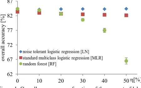
In the first part of this set of experiments, we contaminated the training data by label noise according to the NCAR model. That is, the label noise was assumed to be independent of the class labels, so that the true transition matrix contained identical values ij = 1- for i = j and ij = / (K-1) for i ≠ j, where characterises the percentage of erroneous training labels. Training labels were changed randomly according to that model to simulate label noise. We varied from 0% to 50% in steps of 10%. For training we used 30% of the pixels, which we chose randomly from all available data, taking care to have approximately equal numbers of training samples per class. The RF classifier used for comparison consisted of 300 trees of a maximum depth of 25. A node was split if it contained more than 5 training samples. Each experiment was repeated 20 times, using different training pixels and changing different class labels to simulate label noise. We report the average overall accuracy obtained for all pixels in the scene and also give error bars to indicate maximum and minimum numbers over all 20 test runs per experiment.
The results of the first part of this set of experiments are shown in figure 1. In the absence of label noise, RF delivers slightly better results than both versions of logistic regression, all classifiers achieving an OA of about 84%. With = 10% of wrong labels, RF still delivers results on par with the label noise tolerant logistic regression, but then the OA is decreasing down to 67% for 50% label noise. Standard logistic regression (MLR) turns out to be more robust than RF, with a decrease of only 2-3% even for large amounts of label noise. Label noise robust hand. Some changes in topography are more likely to occur than others, so that the elements of the transition matrix may vary to a larger degree. This is why in the second part of this set of experiments, we simulated label noise according to the NAR model, where the likelihood of a change depends on the class labels. Again we used the variable to characterise the amount of label noise in the training data, but the true transition matrix was generated in a different way. For each row i we randomly selected the probability for each class transition in that row (ij for i ≠ j) so that the sum S = ij ≤ . The element of the main
diagonal was then set to ii = 1- S. Thus, can be interpreted as the maximum percentage of change, and the classes are also affected by change to different degrees. Label noise was simulated according to the transition matrix just described. We varied the values of as in the case of the NCAR experiment, using 30% of the data for training and carrying out 20 tests for each value of . We also varied the transition matrix in each of these tests. To assess the influence of the initial values for the elements of , we carried out a second set of tests for = 50% with label noise tolerant logistic regression based on the initial values ij = 0.5 for i = j and ij = 0.5/ (K-1) for i ≠ j; this version is referred to as version LN50. The overall accuracy values achieved in these experiments are shown in figure 2.
Figure 1. Overall accuracy as a function of the amount of label noise (NCAR model) for three different classifiers.
Figure 2. Overall accuracy as a function of the maximum amount of label noise (NAR model). Note that LN50 was only tested for = 50%.
4%. The experiment with the different initialisation for = 50% (LN50) achieves nearly identical results although one could have expected it to perform better because the initial values are closer to the true ones. This indicates the robustness of the method with respect to the initialisation of .
We cannot give a detailed analysis of completeness and correctness here for lack of space. These quality metrics follow similar trends as the average OA. Buildings and impervious surfaces obtain better quality measures than the other classes, but this observation is independent from the classifier used. In general, the experiments presented in this section indicate that label noise robust logistic regression is well-suited to cope with even relatively large amounts of label noise.
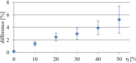
We also analysed the differences between the estimated transition matrices and the true ones that were used to simulate label noise. Figure 3 shows the median of the absolute differences between estimated and true matrix entries for the simulations based on the NAR model. Again we observe that the errors increase with the amount of label noise. For = 50%, the median absolute difference is about 5%, identical to about 10% of the amount of label noise, which we consider to be relatively accurate. The maximum differences, not shown in the figure for lack of space, show a higher rate of increase with increasing amount of label noise. For = 50%, the average maximum error over 20 tests is about 20%.
Figure 3. Median of absolute differences between the estimated and the true elements of the transition matrix (LN).
4.3 Evaluation of Change Detection
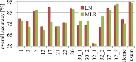
In Section 4.2, the label noise was distributed uniformly in the image, which is not very realistic when considering real changes in topography. For the experiments reported in this section, we simulated realistic changes in all our data sets, changing about 15%-25% of the scene. For three of the Vaihingen test patches we simulated two outdated databases with different distributions of change (cf. figure 4; for Vaihingen we refer to patches by their numbers as given in the benchmark documentation (Wegner et al., 2015), using underscores to differentiate variants of the outdated database. Thus, 30_1 refers to the first variant of the database for patch 30). In this set of experiments, we used all pixels of the outdated database for training and applied the CRF-based classifier to the data. We compare the versions LN and MLR for the association potential of the CRF only to assess the benefits of the version with label noise tolerant training over standard training of logistic regression. The resulting values of overall accuracy for all test areas are presented in figure 5.
Figure 5 shows that the overall accuracy achieved in classification if the label noise robust version of logistic regression is used for the association potential of the CRF (LN) is better than the one for MLR for nearly all the cases. The exceptions are the second variants of the (simulated) outdated databases for areas 30, 32 and 37 in Vaihingen, characterised by
different distributions of label noise in the scene (cf. figure 4 for the difference in area 30). In general, the improvement of LN over MLR is in the order of about 1-2% in Vaihingen. This corresponds to the scenario with approximately 20% label noise observed in Section 4.2, where the differences between these two versions were not yet very pronounced. The improvement of LN over MLR is slightly more obvious for the data sets based on satellite imagery. Note that the disadvantages of MLR may also be mitigated by the smoothing effects due to the CRF. An example for the results achieved by LN is shown in figure 6.
Figure 4. Area 30 in Vaihingen. Left: reference; centre: simulated topographic database (variant 30_1), right: simulated topographic database (variant 30_2). Colours: white: impervious surface; blue: building; green: tree; cyan: low vegetation.
Figure 5. Overall accuracy [%] achieved for all test sites for two versions LN and MLR. Except for Herne and Husum, the numbers are the patch numbers of the Vaihingen data (Wegner et al., 2015).
Figure 6. Vaihingen, area 3. Left: reference; centre: simulated database; right: classification results (LN). The colour code is identical to figure 4.
A typical reason for problems of label noise robust training, occurring in the three cases where MLR achieves a slightly better result than LN, is a change that produces an object that is not represented by the correct training data for that class. An example is the construction of new buildings having an atypical roof material that is not used for any other building in the scene. An analysis of the estimated transition matrices indicates that clusters of atypical pixels that all correspond to label noise can 0
2 4 6 8
0 10 20 30 40 50
d
if
fe
re
n
ce
[
%
]
[%]
75 80 85 90
1 3 5 13 17 21 23 26
30_1 30_2 32_1 32_2 37_1 37_2 Hern
e
Hu
su
m
o
v
era
ll
a
cc
u
ra
cy
[
%
]
cause an overestimation of the off-diagonal elements of these matrices that obviously lead to errors in classification.
Again, we cannot give a detailed analysis of completeness and correctness per class for lack of space; an example, comparing the two versions LN and MLR for all classes except clutter/background (which only occurs in one patch and, thus, is not representative) is shown in figure 7. The figure indicates that there is a different trade-off between type 1 and type 2 errors. However, the quality, being a compound measure integrating both completeness and correctness, is consistently higher for LN than for MLR in this case.
Figure 7. Completeness, correctness and quality per class (bu: building, tr: tree, lv: low vegetation; su: impervious surfaces) for the results in area 3 (Vaihingen). The results for version LN correspond to figure 6 (right).
So far, the evaluation has concentrated on the entire image, thus also integrating unchanged pixels that were also used in the training process. Figure 8 shows the overall accuracy achieved in all tests, only taking into account the pixels affected by a simulated change. In the majority of the examples, LN delivers better results than MLR. The improvement can reach 10% (Vaihingen, area 17), but a more realistic number would be 1-3%, which also applies to the satellite images. In the second variant of changes for area 32 (32_2), where MLR is better than LN by about 5%, there was a large new part of an industrial building with atypical roof material that could not be detected correctly, a problem already discussed above.
Figure 8. Overall accuracy for all tests only taking into account the pixels affected by a change.
Again, we also evaluated the differences between the estimated and the true elements of the transition matrices; figure 9 shows the median of these differences for all tests. In general, the median difference is below 3%, corresponding well to the scenario in figure 3 given the amount of simulated changes. Only the differences for the data set from Husum are atypically large. The median of the differences is about 5.5%. This problem can be attributed to the class rural streets contained in that data set. The maximum error in the transition matrix is related to a transition from rural street to residential, the corresponding probability being estimated as 86% although no such changes were simulated in the data. The estimation of the transition matrix may have been negatively affected by the fact
that only a small number of pixels belongs to class rural streets, which, thus, is underrepresented in the data set.
Figure 9. Median of absolute differences between the estimated and the true elements of the transition matrix (LN).
5. CONCLUSION
In this paper we have presented a method for change detection based on CRF that uses an outdated topographic database to derive training labels for the supervised classification of new data, without any need for training data generated manually. The method takes into account the unavoidable errors in the database by using a model of logistic regression which can deal with label noise. Comparing the classification results with the database, changes having taken place between the original acquisition of the database and the time epoch when the sensor data were acquired.
In our experiments we tested label noise tolerant logistic regression under varying degrees of both, class-independent and class-dependent label noise. In both scenarios label noise tolerant logistic regression delivered very promising results. Even in the presence of up to 50% wrong training labels the classification accuracy was only affected to a small degree compared to a classifier trained on 100% correct labels, whereas the quality of a random forest classifier, supposed to be robust to some degree of label noise, deteriorated by a much larger margin. Applying the CRF-based classification to scenes with simulated realistic changes in the database, the use of label noise tolerant logistic regression for the association potentials increased the classification accuracy over a standard logistic regression for the changed areas by 1-3% in most cases. However, these experiments also showed the limitations of the training method. For instance, we consider the NAR model, which forms the basis of that method, to be too simplistic, neglecting the fact that in our application erroneous training labels occur in local clusters and, thus, are spatially correlated. As far as the estimated transition matrices are concerned, they are reasonably accurate in most cases. However, underrepresented classes or large amounts of label noise may affect the estimation in a negative way.
In our future work we want to expand the model underlying the label noise tolerant classifier so that it can take into account the fact that wrong labels may appear in local clusters. Furthermore, here we used values determined on an empirical basis for the interaction model of the CRF; a joint training procedure similar to the one described in (Kumar & Hebert, 2006) might lead to improved results. We also want to expand our experiments, not restricting ourselves to the relatively small training patches as we did in this paper, so that the problem of atypical objects can be overcome and the results become more representative for different types of imagery. Additionally, we want to expand our experiments to data with real changes instead of simulated ones in order to test our method in a scenario that is more realistic
30_1 30_2 32_1 32_2 37_1 37_2 Hern
e
30_1 30_2 32_1 32_2 37_1 37_2 Hern
with respect to the type and extent of change as well as to the level of detail and number of classes in the existing database.
Finally, we observe that multitemporal classification requires temporal transition probabilities, which are frequently hand-crafted based on heuristic models, e.g. (Hoberg et al., 2015). Our experience with estimating transition matrices presented in this paper gives us reason to believe that our method could be the basis for an empirical estimation of these important model parameters in such a multitemporal context.
ACKNOWLEDGEMENT
The Vaihingen data set was provided by the German Society for Photogrammetry, Remote Sensing and Geoinformation (DGPF) (Cramer, 2010):
http://www.ifp.uni-stuttgart.de/dgpf/DKEP-Allg.html.
REFERENCES
An, W., Liang, M., 2013. Fuzzy support vector machine based on within-class scatter for classification problems with outliers or noises. Neurocomputing 110(2013):101-110.
Bishop, C. M., 2006. Pattern recognition and machine learning. 1st edn, Springer, New York (NY), USA.
Bootkrajang, J., Kabán, A., 2012. Label-noise robust logistic regression and its applications. In: Proceedings of the 2012 European Conference on Machine Learning and Knowledge Discovery in Databases, Vol. I, pp. 143-158
Breiman, L., 2001. Random forests. Machine Learning, 45(1):5–32.
Bruzzone, L., Persello, C., 2009. A novel context-sensitive semisupervised SVM classifier robust to mislabeled training samples. IEEE Transactions on Geoscience and Remote Sensing 47(7):2142-2154.
Büschenfeld, T., 2013. Klassifikation von Satellitenbildern unter Ausnutzung von Klassifikationsunsicherheiten. PhD thesis, Fortschritt-Berichte VDI, Reihe 10 Informatik / Kommunikation, Vol. 828, Institute of Information Processing, Leibniz Universität Hannover, Germany.
Champion, N., 2007. 2D Building change detection from high resolution aerial images and correlation digital surface models. International Archives of the Photogrammetry, Remote Sensing and Spatial Information Sciences Vol. XXXVI-3 / W49A, pp. 197-202.
Cramer, M., 2010. The DGPF test on digital aerial camera evaluation – overview and test design. Photogrammetrie Fernerkundung Geoinformation 2(2010):73–82.
Frénay, B., Verleysen, M., 2014. Classification in the presence of label noise: a survey. IEEE Transactions on Neural Networks on Learning Systems 25(5):845-869.
Frey, B. J., MacKay, D. J. C., 1998. A revolution: belief propagation in graphs with cycles. In: Proceedings of the Neural Information Processing Systems Conference, pp. 479– 485.
Hoberg, T., Rottensteiner, F., Feitosa, R. Q., Heipke, C., 2015. Conditional random fields for multitemporal and multiscale classification of optical satellite imagery. IEEE Transactions on Geosciences and Remote Sensing 53(2):659-673.
Jia, K., Liang, S., Wei, X., Zhang, L., Yao, Y., Gao, S., 2014. Automatic land-cover update approach integrating iterative traing sample selection and a markov random field model. Remote Sensing Letters 5(2):148-156.
Jianya, G., Haigang, S., Guorui, M., Qiming, Z., 2008. A review of multi temporal remote sensing data change detection algorithms. The International Archives of the Photogrammetry, Remote Sensing and Spatial Information Sciences XXXVII-B7, pp. 757-762.
Kumar, S., Hebert, M., 2006. Discriminative random fields. International Journal of Computer Vision 68(2): 179-201.
Li, Y., Wessels, L. F. A., de Ridder, D., Reinders, M. J. T., 2007. Classification in the presence of class noise using a probabilistic kernel Fisher method. Pattern Recognition 40(2007):3349-3357.
Lu, D., Mausel, P., Brondizio, E., Moran, E., 2004. Change detection techniques. International Journal of Remote Sensing 25(12):2365-2401.
Mnih, V., Hinton, G., 2012. Learning to label aerial images from noisy data. In: Proc. 29th International Conference on Machine Learning, pp. 567-574.
Radoux, J., Defourny, P., 2010. Automated image-to-map discrepancy detection using iterative trimming. Photo-grammetric Engineering & Remote Sensing 76(2):173-181.
Radoux, J., Lamarche, C., Van Bogaert, E., Bontemps, S., Brockmann, C., Defourny, P., 2014. Automated training sample extraction for global land cover mapping. Remote sensing 6(2014):3965-3987.
Rutzinger, M., Rottensteiner, F. and Pfeifer, N., 2009. A comparison of evaluation techniques for building extraction from airborne laser scanning. IEEE Journal of Selected Topics in Applied Earth Observation and Remote Sensing 2(1):11-20.
Shotton, J., Winn, J., Rother, C., and Criminisi, A., 2009. Textonboost for image understanding: Multi-class object recognition and segmentation by jointly modeling texture, layout, and context. International Journal of Computer Vision, 81(1): 2–23.
Subudhi, B. N., Bovolo, F., Ghosh, A., Bruzzone, L., 2014. spatio-contextual fuzzy clustering with markov random field model for change detection in remotely sensed images. Optics and Laser Technology 57(2014):284-292.
Vosselman, G., Gorte, B., Sithole, G., 2004. Change detection for updating medium scale maps using laser altimetry. International Archives of the Photogrammetry, Remote Sensing and Spatial Information Sciences vol XXXV-B3, pp. 207-212.
Wegner, J.D., Rottensteiner, F., Gerke, M., Sohn, G., 2015. The
ISPRS 2D Labelling Challange.