SEMANTIC SEGMENTATION OF AERIAL IMAGES WITH AN ENSEMBLE OF CNNS
D. Marmanisa,d, J. D. Wegnera, S. Gallianib, K. Schindlerb, M. Datcuc, U. Stillad
aDLR-DFD Department, German Aerospace Center, Oberpfaffenhofen, Germany – [email protected] b
Photogrammetry and Remote Sensing, ETH Zurich, Switzerland –{jan.wegner, silvano.galliani, schindler}@geod.baug.ethz.ch c
DLR-IMF Department, German Aerospace Center, Oberpfaffenhofen, Germany – [email protected] dPhotogrammetry and Remote Sensing, TU M¨unchen, Germany – [email protected]
ICWG III/VII
ABSTRACT:
This paper describes a deep learning approach to semantic segmentation of very high resolution (aerial) images. Deep neural architec-tures hold the promise of end-to-end learning from raw images, making heuristic feature design obsolete. Over the last decade this idea has seen a revival, and in recent years deep convolutional neural networks (CNNs) have emerged as the method of choice for a range of image interpretation tasks like visual recognition and object detection. Still, standard CNNs do not lend themselves to per-pixel semantic segmentation, mainly because one of their fundamental principles is to gradually aggregate information over larger and larger image regions, making it hard to disentangle contributions from different pixels. Very recently two extensions of the CNN framework have made it possible to trace the semantic information back to a precise pixel position: deconvolutional network layers undo the spatial downsampling, and Fully Convolution Networks (FCNs) modify the fully connected classification layers of the network in such a way that the location of individual activations remains explicit. We design a FCN which takes as input intensity and range data and, with the help of aggressive deconvolution and recycling of early network layers, converts them into a pixelwise classification at full resolution. We discuss design choices and intricacies of such a network, and demonstrate that an ensemble of several networks achieves excellent results on challenging data such as theISPRS semantic labeling benchmark, using only the raw data as input.
1. INTRODUCTION
Large amounts of very high resolution (VHR) remote sensing im-ages are acquired daily with either airborne or spaceborne plat-forms, mainly as base data for mapping and earth observation. Despite decades of research the degree of automation for map generation and updating still remains low. In practice, most maps are still drawn manually, with varying degree of support from semi-automated tools [Helmholz et al., 2012]. What makes au-tomation particularly challenging for VHR images is that on the one hand their spectral resolution is inherently lower, on the other hand small objects and small-scale surface texture become visi-ble. Together, this leads to high within-class variability of the im-age intensities, and at the same time low inter-class differences.
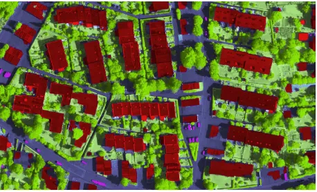
An intermediate step between raw images and a map layer in vec-tor format is semantic image segmentation (a.k.a. land-cover clas-sification, or pixel labeling). Its aim is to determine, at every im-age pixel, the most likely class label from a finite set of possible labels, corresponding to the desired object categories in the map, see Fig. 1. Semantic segmentation in urban areas poses the addi-tional challenge that many man-made object categories are com-posed of a large number of different materials, and that objects in cities (such as buildings or trees) are small and interact with each other through occlusions, cast shadows, inter-reflections, etc.
A standard formulation of the semantic segmentation problem is to cast it as supervised learning: given some labeled training data, a statistical classifier learns to predict the conditional probabili-tiesgi=P(class=i|data)from spectral features of the image. Typical choices of input features are raw pixel intensities, simple arithmetic combinations of the raw values such as vegetation in-dices, and different statistics or filter responses that describe the local image texture [Leung and Malik, 2001, Schmid, 2001, Shot-ton et al., 2009]. Since the advent of classifiers that include effi-cient feature selection (e.g., boosting, decision trees and forests), an alternative has been to pre-compute a large, redundant set of
Figure 1: Class map estimated with the proposed ensemble of fully convolution networks (FCNs), over a scene taken from un-labelled officialISPRS Vaihingendataset. Visualization is color coded, red color depictsbuildings, dark green depictstrees, light green depicts low-vegetation, blue depicts impervious-surfaces and purple depictscarsrespectively.
features for training and let the classifier select the optimal sub-set [Viola and Jones, 2001, Doll´ar et al., 2009, Fr¨ohlich et al., 2013, Tokarczyk et al., 2015], in the hope that in this way less of the relevant information is lost by the feature encoding.
al., 2015], if given enough training data and compute power. CNNs on one hand exploit the shift-invariance of image signals, on the other hand they can easily be parallelised and run on GPUs, making it possible to train from millions of images on a sin-gle machine. In recent years they have been the top-performing method for tasks ranging from speech processing to visual ob-ject recognition. Recently, CNNs have also been among the top performers on the ISPRS benchmark for aerial image labelling1, e.g., [Paisitkriangkrai et al., 2015]. For completeness, we note that earlier deep learning methods have also occasionally been applied for remote sensing, e.g. [Mnih and Hinton, 2010].
In this paper, we explore the potential of CNNs for end-to-end, fully automated semantic segmentation of high-resolution images with<10cm ground sampling distance. Starting from their per-pixel classifier version, so-calledFully Convolutional Networks (FCNs), we discuss a number of difficulties, and propose de-sign choices to address them. In particular, we employ a late fusion approach with two structurally identical, parallel process-ing strands within the network, in order to use both image in-tensities and DEM data as input, while respecting their differ-ent statistical characteristics. We also show that model averaging over multiple instances of the same CNN architecture, trained with different initial values for the (millions of) free parameters in the network, even further improves the final segmentation result. Compared to other work on FCNs in remote sensing [Paisitkri-angkrai et al., 2015, Lagrange and Le Saux, 2015], we employ strictly end-to-end training and refrain from using any informa-tion that requires manual interacinforma-tion, such as hand-designed filter responses, edges or normalised DSMs. Experiments on the IS-PRSVaihingenDataset show that our method achieves state-of-the-art results, with overall accuracy>88% on unseen test data.
2. RELATED WORK
Much research effort has gone into semantic segmentation of satel-lite and aerial images in the last three decades. For a general background we refer the reader to textbooks such as [Richards, 2013]. Here, we review some of the latest works dealing with very high-resolution (VHR) imagery, which we define as having a GSD on the order of10cm. We then turn to recent advances in general image analysis with deep learning methods. VHR data calls for different strategies than lower-resolution images (such as the often-used Landsat and SPOT satellite data), due to the in-comparably greater geometric detail; and, conversely, the much lower spectral resolution – in most cases only RGB channels, and possibly an additional NIR.
In VHR data the class information is not sufficiently captured by a pixel’s individual spectral intensity, instead analysis of tex-ture and spatial context becomes important. Consequently, much of the literature has concentrated on feature extraction from a pixel’s spatial neighborhood [Herold et al., 2003, Dalla Mura et al., 2010, Tokarczyk et al., 2015]. As in other areas of image analysis, too [Winn et al., 2005], the emphasis was on finding (by trial-and-error) a feature encoding that captures as much as pos-sible of the relevant information, while ideally also being com-putationally efficient. The features are then fed to some standard classification algorithm (SVM, Random Forest, logistic regres-sion or similar) to predict class probabilities. As local feature engineering began to saturate, more emphasis was put on includ-ing a-priori information about the class layout like smoothness, shape templates, and long-range connectivity [Karantzalos and
1
http://www2.isprs.org/commissions/comm3/wg4/ semantic-labeling.html
Paragios, 2009, Lafarge et al., 2010, Schindler, 2012, Montoya-Zegarra et al., 2015], often in the form of Conditional Random Fields or Marked Point Processes.
In the last few years neural networks, which had fallen out of favour in machine learning for some time, have made a spectac-ular return. Driven by a number of methodological advances, but especially by the availability of much larger image databases and fast computers, deep learning methods – in particular CNNs – have outperformed all competing methods on several visual learning tasks. With deep learning, the division into feature ex-traction, per-pixel classification, and context modelling becomes largely meaningless. Rather, a typical deep network will take as input a raw image. The intensity values are passed through mul-tiple layers of processing, which transform them and aggregate them over progressively larger contextual neighborhoods, in such a way that the information becomes explicit which is required to discriminate different object categories. The entire set of network parameters is learned from raw data and labels, including lower layers that can be interpreted as “features”, middle layers that can be seen as the “layout and context” knowledge for the specific do-main, and deep layers that perform the actual “classification”.
Among the first who applied CNNs to semantic segmentation were [Farabet et al., 2013], who label super-pixels derived from a large segmentation tree. In the course of the last year multiple works have pushed the idea further. [Chen et al., 2015] propose to add a fully connected CRF on top of a CNN, which helps to re-cover small details that get washed out by the spatial aggregation. Similarly, [Tsogkas et al., 2015] combine a CNN with a fully con-nected CRF, but add a Restricted Boltzmann Machine to learn high-level prior information about objects, which was previously lacking. The top-performers for semantic segmentation of remote sensing images are based on CNNs, too. [Lagrange et al., 2015], ranked second in the 2015 2D IEEE GRSS data fusion contest, use pre-trained CNNs as feature extractor for land cover classi-fication. More similar to our research is the work of [Paisitkri-angkrai et al., 2015], who are among the top performers on the ISPRS semantic segmentation benchmark. Instead of directly applying pre-trained models, the authors individually train a set of relatively small CNNs over the same aerial images (respec-tively, nDSMs) with different contextual input dimensions. Re-sults are further refined with an edge-sensitive, binary CRF. In contrast to those works, which make use of several ad-hoc pre-and post-processing steps (e.g., extraction of vegetation indices; terrain/off-terrain filtering of the DSM; additional Random For-est classifier), we attempt to push the deep learning philosophy to its extreme, and construct a true end-to-end processing pipeline from raw image and DSM data to per-pixel class likelihoods.
3. SEMANTIC SEGMENTATION WITH CNNS
ConvolutionalNeural Networks are at present the most success-ful deep learning architecture for semantic image understanding tasks. Their common property is the use of layers that implement learned convolution filters: each neuron at level ltakes its in-put values only from a fixed-size, spatially localised windowW in the previous layer(l−1), and outputs a vector of differently weighted sums of those values,cl=P
i∈Wwic l−1
i . The weights wifor each vector dimension are shared across all neurons of a layer. This design takes into account the shift invariance of image structures, and greatly reduces the number of free parameters in the model.
Each convolutional layer is followed by a fixed non-linear trans-formation2, in modern CNNs often a rectified linear unit (ReLU)
2
cl
rec = max(0, cl), which simply truncates all negative values to 0and leaves the positives values unchanged [Nair and Hin-ton, 2010]. Moreover, the network also gradually downsamples the input spatially, either by using a stride> 1for the convo-lutions or with explicit spatialpooling layers. By doing so, the network gradually increases its receptive field, collecting infor-mation from a larger spatial context. Finally, the top layers of the model are normally fully connected to combine information from the entire image, and the final output is converted to class probabilities with thesof tmaxfunction.
CNNs can be learned end-to-end in a supervised manner with the back-propagation algorithm, usually using stochastic gradients in small batches for efficiency. In the last few years they have been extremely successful and caused a small revolution in the fields of speech and image analysis.
Fully Convolutional Neural Networks CNNs in their original form were designed forrecognition, i.e. assigning a single label (like “car” or “dog”) to an entire image. The bottleneck when us-ing them for semantic segmentation (labelus-ing every sus-ingle pixel) is the loss of the spatial location. On the one hand, repeated con-volution and pooling smear out the spatial information and re-duce its resolution. On the other hand, even more severe, fully connected layers mix the information from the entire image to generate their output.
In recent work [Zeiler et al., 2010, Long et al., 2015], extensions of the basic CNN architecture have been developed, which mit-igate this problem, but still allow for end-to-end learning from raw images to classification maps. So-calledFully Convolutional Networksview the fully connected layers as a large set of1×1 convolutions, such that one can track back the activations at dif-ferent image locations. Moreover,deconvolution layersthat learn to reverse the down-sampling, together withdirect connections from lower layersthat “skip” parts of network, make it possible to predict at a finer spatial resolution than would be possible after multiple rounds of pooling.
Converting a CNN into a FCN Traditional CNN architectures for image-level classification (like the popular variantsOverFeat, AlexNet, GoogLeNet, VGGnet) do not aim for pixel-level seg-mentation. They require an input image of fixed sizew×hand completely discard the spatial information in the top-most layers. These are fully connected and output a vector of class scoresgi. FCNs use the following trick to trace back the spatial location: the fully connected layers are seen as convolution with aw×h kernel, followed by a large set of1×1convolutions that generate a spatially explicit map of class scoresgi(x, y). Since all other layers correspond to local filters anyway, the network can then be applied to images of arbitrary size to obtain such a score map.
Deconvolution layers The FCN outputs per-class probability maps, but these come at an overly coarse spatial resolution, due to the repeated pooling in the lower layers. The FCN is thus augmented with deconvolution layers, which perform a learned upsampling of the previous layer. I.e., they are the reverse of a convolution layer (literally, backpropagation through such a layer amounts to convolution). By inserting multiple deconvolution layers in the upper parts of the network, the representation is upsampled back to the original resolution, so as to obtain class scores for each individual pixel.
Deconvolution layers are notoriously tricky to train. We follow the current best practice and employdeep supervision[Lee et al., 2014]. The idea is to add “shortcuts” from intermediate layers
since it is equivalent to a single convolution with the new kernelv ⋆ u.
directly to a classification layer and associated additional com-panion loss functions. Bypassing the higher layers provides a more direct supervision signal to the intermediate layers. It also mitigates the problem that small gradients vanish during back-propagation and speeds up the training.
Reinjecting low-level information The deconvolution layers bring the representation back to the full resolution. But they do not have access to the original high-frequency information, so the best one can hope for is to learn a good a-priori model for upsam-pling. To recover finer detail of the class boundaries, one must go back to a feature representation near the original input resolution. To do so, it is possible, after a deconvolution layer, to combine the result with the output of an earlier convolution layer of the same spatial resolution. These additional “skip” connections by-pass the part of the network that would drop the high-frequency information. The original, linear sequence of operations is turned into a directed acyclic graph (DAG), thus giving the classification layers at the top access to high-resolution image details.
Training Multiple CNNs Deep networks are notorious for hav-ing extremely non-convex, high-dimensional loss functions with many local minima.3If one initialises with different (pre-trained, see next paragraph) sets of parameters, the net is therefore vir-tually guaranteed to converge to different solutions, even though it sees the same training data. This observation suggests a sim-ple model averaging (ensemble learning) procedure: train several networks with different initialisations, and average their predic-tions. Our results indicate that, as observed previously for image-level classification, e.g. [Simonyan and Zisserman, 2015], aver-aging multiple CNN instances further boosts performance.
Note that model averaging in the case of end-to-end trained deep networks is in some sense a “stronger” ensemble than if one av-erages conventional classifiers such as decision trees: all classi-fiers in a conventional ensemble work with the same predefined pool of features, and must be decorrelated by randomising the feature subset and/or the training algorithm (c.f. the popular Ran-dom Forest method). On the contrary, CNNslearnuseful features from the raw data, thus even the low-level features in early layers can be expected to vary across different networks and add diver-sity to the ensemble.
We also point out that while it might seem a big effort to train multiple complicated deep networks, it is in fact very simple. Training only needs raw images and label maps as input, and a small number of hyper-parameters such as the learning rate and its decay. Since the variation comes from the initialization, one need not to change anything in the training procedure, but merely has to rerun it multiple times.
Pre-trained Networks The most powerful CNN models for im-age analysis have been trained over many iterations, using huge databases with thousands or even millions of images. Fortunately, it turned out that CNNs are good at transfer learning: once a network has been trained with a large database, it has adapted well enough to the structure of image data in general, so that it can be adapted for a new task with relatively little training. It is now common practice to start from an existing network that has been pre-trained on one of the big image databases such as Im-ageNet[Russakovsky et al., 2015],Microsoft COCO[Lin et al., 2014],Pascal VOC[Everingham et al., 2010], etc. In this way, the network only needs to be fine-tuned to the task at hand, which requires a lot less training data and computation time.
3
Local minimumdoes not equate tobad solutionhere. There is no
For remote sensing application, it is at present still unclear which of the existing pre-trained models is most suitable. In fact, it is quite likely that none of them is optimal. On the other hand, it is also not clear what would be a better architecture for remote sensing problems, and how to chose the right (big) dataset to train it from scratch. Our solution at this point is to start from several proven networks that have excelled in other applications, and apply model averaging to combine their results. In particular we use the following three networks to initialize three separate FCNs: VGG-16, trained on ImageNet; FCN-Pascal, trained on Pascal VOC specifically for semantic segmentation; andPlaces, trained on the MIT Places database for scene recognition.
TheVGG-16network was designed for theImageNet 2012 Large-Scale Visual Recognition Challenge, and achieved excellent over-all results [Simonyan and Zisserman, 2015]. Important character-istics of the VGG architecture are relatively few trainable param-eters per layer, due to the use of small convolution kernels of size 3×3. This makes it possible to train very deep networks with 16 (or even 19) layers in reasonable time. For our task of seman-tic segmentation, we convert the 16-layer version to a FCN. This proved to be the strongest individual network for our data.
TheFCN-Pascalnetwork is another powerful network pre-trained on thePascal VOC Contextdatabase for the purpose of semantic segmentation [Long et al., 2015]. Its lower layers have the same layout as VGG-16, but it already comes as fully connected net-work for pixel-wise labeling, so it is arguably most tuned to our application. We point out that this network is not completely in-dependent of the previous one, because its creators started from VGG-16 and transferred it to the Pascal VOC database. In our implementation, we start from the final version optimized for Pas-cal VOC, and further adapt it to our aerial images. An interesting feature of FCN-Pascal is the cascaded training procedure, which starts from a shallower, partial model and gradually adds layers so as to learn the DAG-connections from low convolutional layers to high deconvolutional ones. We also employ a set of 4 cascaded architectures when training this particular model. Empirically, the final, deepest model works better than any of the intermediate shallower ones, so we only use the latest one in our final classifier.
ThePlacesNetwork also uses the VGG-16 architecture, but has been learned from scratch on a different dataset. Its training set is a scene recognition dataset namedPlaces[Zhou et al., 2014]. We expect this model to be less correlated to the other two, so that it can make a contribution during model averaging, although by itself it has significantly lower performance on our data.
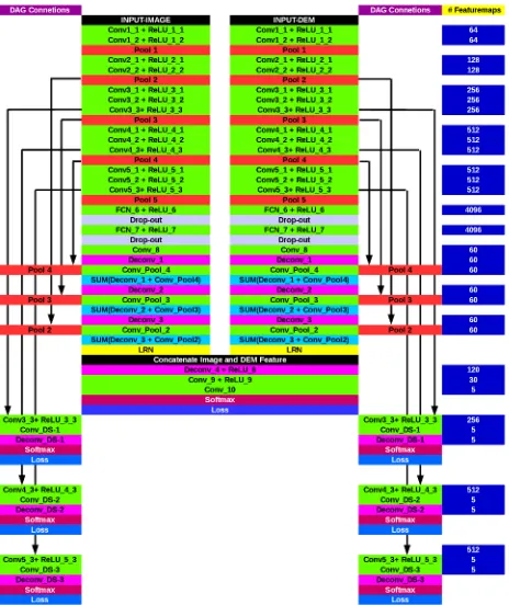
Complete Network Architecture Our network is an extension of theFCN-Pascalnetwork introduced above, see Fig. 2. It uses small3×3convolution kernels throughout. Compared to the original layout we add another skip-layer connection to inject high-resolution features from an even earlier layer, in order to better represent the fine detail of the class boundaries. Moreover, we use as input not only the image intensities but also the DEM, as often done in high-resolution remote sensing. Since height data and intensity data have different statistics, one should expect that they require different feature representations. We therefore set up two separate paths for the two modalities with the same layer architecture, and only merge those two paths at a very high level, shortly before the final layer that outputs the class prob-abilities. This late fusion of spectral and height features makes it possible to separately normalise spectral and height responses (see next paragraph), and shall enable the network to learn inde-pendent sets of meaningful features for the two inputs, driven by the same loss function.
The last modification of the FCN network is of a technical na-ture. We found that the network during training exhibited a
ten-Figure 2: Schematic diagram of our network architecture. Layers and connections on the left, number of kernels per layer on the right. All convolution kernels are3×3, all max-pooling windows are2×2, with no overlap.
dency to excessively increase the activations at a small number of neurons. To prevent the formation of such spikes, whose exag-gerated influence causes the training to stall, we add local re-sponse normalisation (LRN) as last layer of the two separate branches for spectral intensities and height, right before merging them for the final classification stage. LRN was first employed by [Krizhevsky et al., 2012] and can be biologically interpreted aslateral inhibition. It amounts to re-scaling activations, such that spikes are damped and do not overly distort the gradients for back-propagation. The LRN for an activationcis defined as cLRN =c· 1 +αP
i∈Nγc 2
i −β
, with hyper-parametersαand β, andNγ a neighborhood ofγ “adjacent” kernels at the same spatial location (although the ordering of the kernels is of course arbitrary). We setγ= 5, and choseαandβsuch that intensity and DEM activations are both scaled to mean values of≈10.
Implementation Details While CNNs offer end-to-end machine learning and empirically obtain excellent results, training them does require some care. In our network, the part that appears hardest to learn are the deconvolution layers. We initialise the upsampling weights with bilinear interpolation coefficients and use deep supervision, nevertheless these layers slow down the back-propagation and require many training iterations.
Local Response Normalizationproved to be crucial. We assert that there are two main reasons (both not specific to our model). First,ReLUnon-linearities are not bounded from above, so there is no built-in saturation that would stop the formation of spikes.4 Second, the initial input data is not whitened (mainly for practi-cal reasons, because of its large volume). We found that spikes did hold back the training of our network and therefore introduce
4
LRN layers at the appropriate stages, where the effect occurs. For a given architecture and data characteristics this solves the prob-lem once and for all, but we note that when faced with a different problem it may be important to check the activation statistics and insert LRN where necessary.
In our experience, a good practice with large, pre-trained CNNs isgradual training, starting from the deeper layers. The low-level features, while not fully optimised to the task at hand, can be assumed to already be reasonable, so we first clamp them and only update the deep layers of the network near the output, which are initially tuned to the completely different class nomenclature of the pre-training task. When the loss flattens out, or after a fixed number of iterations, one adds further layers, until finally the full network is optimised. This greatly speeds up the training.
4. EXPERIMENTS
We empirically validate our approach with experiments on the Vaihingen data set of the ISPRS 2D semantic labeling contest. It comprises 33 tiles, varying a bit in size, from an aerial orthophoto mosaic with three spectral bands (red, green, near-infrared), plus a digital surface model (DSM) of the same resolution. The data set contains roughly1.7×108
pixels in total, but ground truth is only released for half of the tiles, which are designated for training and validation. For the remainder, the ground truth is withheld by the organizers for objective evaluation of submitted results. The images are rich in detail, with a GSD of9cm. Cat-egories to be classified areImpervious Surfaces, Buildings, Low Vegetation, Trees, and Cars. In order to keep our pipeline au-tomated to the largest possible degree, we refrain from any pre-processing that would require human intervention or selection of data-specific hyper-parameters (such as DSM-to-DTM filtering, or radiometric adjustments), but rather feed the data provided by the benchmark directly into the network.
For our detailed experiments, we split those 16 tiles, for which ground truth is available, into a training subset (tile numbers 1, 3, 11, 13, 15, 17, 21 ,26, 28, 32, 34, 37) and a hold-out subset for testing (tiles 5, 7, 23, 30). We randomly sample 12,000 patches of259×259pixels from the training subset for learning the FCN parameters. Note that also at test time the network outputs labels for a complete patch of259×259pixels at once. To predict labels for whole tiles, we run it on overlapping patches and average the per-pixel class scores.
Training Details Low-level features like edges or colors do not vary dramatically across different images, while the high-level features that capture larger shapes and patterns are more task-specific. Thus it makes sense to first train only the deep layers, while keeping the shallower ones fixed. We first train all layers above the fully-convolutional ones (see Fig. 2) for 40’000 epochs, then train the entire model for another 50’000 epochs. Empiri-cally, the latter only marginally increases the performance (gain in overall accuracy<1%), which indicates that the filter weights of lower layers indeed generalise from close-range images to re-mote sensing imagery. It is common practice to start with a rea-sonably fast learning rate, and keep decreasing it during training. In this way, the network learns faster in the beginning, when it is still far from a good solution, but does not overshoot when fine-tuning in the end. We start with a learning rate oflr = 10−9
, and reduce it by a factor of10every 20,000 epochs.
Each training iteration consists of a feed-forward pass, a com-parison between the prediction and the ground truth labels, and a back-propagation step, in which the weights in the network are adjusted via Stochastic Gradient Descent. Forward passes
require only matrix multiplications and are a lot cheaper than back-propagation, where gradients have to be evaluated for all the weights.
It is also good practice to use so-calleddrop-outduring training, i.e., randomly switch off part of the neurons to decorrelate the learning of different neurons and reduce over-fitting. We use a 50% drop-out rate at two deep layers, as shown in Fig. 2. Em-pirically, we find that in our case drop-out during training only marginally increases performance. We attribute this to two rea-sons. First, the models we start from have already been care-fully pre-trained (with drop-out) on large databases. The (shal-lower) majority of layers is fine-tuned to our training data, but not dramatically altered w.r.t. the initial, well-regularised state, so that over-fitting is not an issue. Second, our model includes direct connections from shallow to deep layers. The purpose of these “skip” connections is better spatial localisation, but it is possible that merging in the low-level features, which are more generic and less prone to over-fitting, also regularises the more task-specific high-level patterns.
FCRF Post-processing As mentioned earlier, the focus of this work lies on an integrated deep-learning approach. Neverthe-less, it is of course possible to view FCN predictions as pixel-wise unary likelihoods and post-process them with CRF-type pri-ors. Some authors have tried this and have shown that it (moder-ately) improves aerial image segmentation [Paisitkriangkrai et al., 2015]. To quantify the influence of state-of-the-art post process-ing we therefore optionally use the class likelihoods predicted by our FCN ensemble as input to a fully connected CRF (FCRF) [Kr¨ahenb¨uhl and Koltun, 2011], similar to [Chen et al., 2015, Zheng et al., 2015]. Most work in remote sensing uses a CRF with pairwise potentials only between neighbouring pixels. The fully connectedCRF does not seem to be widely used, the only example we know of is [Quang et al., 2015]. But but we found it to work better than a standard pairwise CRF.
The prior brings only a tiny quantitative improvement, even if carefully tuned for optimum (overall) performance. It does how-ever qualitatively improve object boundaries, see examples in Fig. 3. Without a deeper analysis, we assert that there is sim-ply not much to be gained, because the FCN already learns to take into account the context within a259×259pixel window. Differences occur mainly in the form of small, isolated regions near class boundaries. There, the smoothing learned by the FCN seems to be a little bit weaker than it should be, such that isolated mis-classifications survive. In the following, we always quote re-sults both without and with FCRF post-processing, but we note that the quantitative differences are insignificant, except for a ten-dency to smooth away cars in favour of the surrounding road.
4.1 Results
In the following we name models according to the data set used for pre-training model weights. Recall that the network architec-ture is the same for all models. FCN-Pascal of [Long et al., 2015] was pre-trained on Pascal VOC, FCN-ImageNet of [Simonyan and Zisserman, 2015] was pre-trained on the ImageNet data set, and FCN-Places of [Zhou et al., 2014] was pre-trained on the Places data set. All models are fine-tuned on our aerial data with-out any changes to their network architectures.
FCN-ImageNet+FCN-Pascal+FCN-Places tile 5 tile 7 tile 23 tile 30 Mean
FCN 86.6 87.2 83.7 85.5 85.7
FCN-ImageNet+FCN-Pascal
FCN 86.3 87.1 83.7 86.1 85.8
FCN-FCRF 86.8 86.9 84.2 86.2 86.0
FCN-ImageNet
FCN 85.2 86.8 82.8 85.6 85.1
FCN-Pascal
FCN 84.7 86.2 82.4 85.2 84.6
FCN-Places
FCN 84.0 82.1 77.5 77.2 80.2
Table 1: Overall accuracies over the four images of our hold-out set. The fully connected CRF (FCN-FCRF) is only tested with the top-performing FCN ensemble (FCN-ImageNet+FCN-Pascal). We report overall accuracies per scene, and average over-all accuracy across over-all four scenes (over-all numbers in %).
FCN
Imp. Surf. 93.1 1.8 3.8 1.1 0.2 Building 7.2 89.1 3.3 0.3 0.1 Low Veg. 4.0 1.6 81.3 13.0 0
Tree 0.7 0.2 6.8 92.3 0 Car 19.4 4.9 0.5 0.4 74.8
Overall Accuracy :88.4
FCN-FCRF
Imp. Surf. 93.6 1.7 3.6 1.0 0.1 Building 7.1 89.4 3.3 0.3 0.1 Low Veg. 3.9 1.6 81.8 12.7 0
Tree 0.8 0.2 7.0 92.0 0 Car 28.1 4.8 0.6 0.4 66.1
Overall Accuracy :88.5
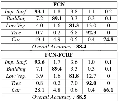
Table 2: Confusion matrices and overall accuracies for the test set of the ISPRS benchmark (all numbers in %).
separate results per model are given. Recall that classifier scores of different models are always combined by averaging prediction scores across models per class.
To further clean up isolated, mis-classified pixels and to sharpen edges we add the fully connected CRF (FCRF) of [Kr¨ahenb¨uhl and Koltun, 2011] on top of the best performing ensemble FCN (FCN-ImageNet+FCN-Pascal) and report quantitative results in Tab. 1. In general, the FCRF only marginally improves the num-ber, but it does visually improve results (Fig. 3).
It turns out that pre-training weights on the Places data set (FCN-Places) performs worst among the three models (bottom rows in Tab. 1) if applied stand-alone to the Vaihingen data. Furthermore, adding it to the ensemble slightly decreases mean overall accura-cies on the hold out subset (by0.04percent points) compared to ImageNet+Pascal (Tab. 1). Pascal and FCN-ImageNet deliver similarly good results, and their combination slightly improves over the separate models.
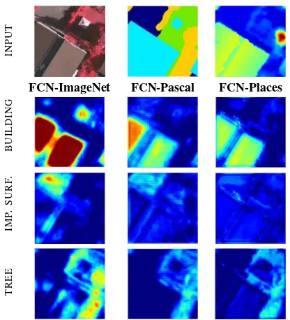
Fig. 4 visually compares the output scores of all three models for four classes (red: high score, blue: low score). FCN-ImageNet generally shows the highest activations thus discriminating classes best, cf. Tab. 1. Each model assigns slightly different class scores per pixel, such that they can complement another.
We also submitted the results of the best performing FCN en-semble (FCN-ImageNet+FCN-Pascal) and its FCN-FCRF vari-ant to the ISPRS 2D semvari-antic labeling test.5 On the test set (for
5
www2.isprs.org/vaihingen-2d-semantic-labeling-contest.html
IM
A
G
E
L
A
B
E
L
S
F
C
N
F
C
N
-F
C
R
F
Figure 3: Comparison of FCN with FCN-FCRF outputs on tiles.
which the ground truth is not public) we reach 88.4% overall accuracy with the FCN ensemble alone, and88.5% with FCRF post-processing, see Tab. 2. I.e., we reach the second best over-all result,0.6percent points below the top-performing method. Moreover, our method works particularly well on the smallertree andcarclasses and, with86.9%, reaches the highest averageF1 -score, 1 percent point higher than the nearest competitor. We note that compared to other methods we do not use a normalised DSM as additional input. The nDSM seems to be a key ingredi-ent for the performance of some methods, c.f. [Paisitkriangkrai et al., 2015], and can be expected to also improve our results. But generating it via DSM-to-DTM filtering requires dataset-specific parameters, which we want to avoid. We also do not add conven-tional classifiers such as Random Forests in our ensemble, be-cause they wold require manual feature engineering.
4.2 Discussion
IN
P
U
T
FCN-ImageNet FCN-Pascal FCN-Places
B
U
IL
D
IN
G
IM
P
.
S
U
R
F
.
T
R
E
E
Figure 4: Score maps for classesbuilding,impervious surface, low vegetation, andtreeof the three pre-trained models using the input in the top row (red: high score, blue: low score).
part be caused by the features’ increased location uncertainty af-ter pooling and deconvolution. We assert that a further reason could be the inherent inaccuracy of the annotated training data. Human annotators with their domain knowledge will usually an-notate a sharp and straight boundary, but they might not be as consistent in placing it w.r.t. the image gradient. If in different patches the same class boundaries are randomly shifted inwards or outwards by a few pixels, this could cause the system to “learn” that uncertainty in the boundary localisation. In true ortho-photos the boundaries are particularly difficult to define precisely, as lim-ited DSM accuracy often causes small parts of facades to be visi-ble near the roof edge, or the roof edge to visi-bleed into the adjacent ground (c.f. Fig. 4).
Another more technical problem that currently limits performance is the restricted receptive field of the classifier. We choose259× 259pixel patches over which the classifier assigns class proba-bilities per pixel. Increasing the window size leads to a massive increase in unknowns for the fully convolutional layers, which eventually makes training infeasible. This is particularly true for remote sensing, where images routinely have many millions of pixels and one cannot hope to overcome the limitation by brute computational power. Tiling will at some point be necessary. We make predictions in a sliding window fashion with overlap-ping patches (of one or multiple different strides) and average the scores from different patches for the final score map. An ap-propriate stride is a compromise between computational cost and sufficient coverage. Moreover, it makes sense to use multiple dif-ferent strides or some degree of randomisation, in order to avoid aliasing. The extreme case of a one-pixel stride (corresponding to 67’081 predictions per pixel) will lead to much computational overhead without significant performance gain, since neighbor-ing predictions are highly correlated. On the other hand, tilneighbor-ing images without any overlap will lead to strong boundary effects. What is more, the spatial context would be extremely skewed for pixels on the patch boundary – in general one can assume that the classifier is more certain in the patch center. For our final model we empirically found that overlapping predictions with a small number of different strides (we use 150, 200and 220pixels) produces good results, while being fast to compute. The over-all classification time for a new scene (2000x2500pixel) using
image ground truth prediction
Figure 5: Labeling errors in the ground truth.
two networks (FCN-ImageNet , FCN-Pascal) with three different strides is≈9minutes with a single GPU. Additional FCRF infer-ence takes≈9minutes per scene on a single CPU, but multi-core parallelisation across different scenes is trivial.
Limitations of the ground truth A close inspection of the an-notations for the Vaihingen data set quickly reveals a number of ground truth errors (as also noticed by [Paisitkriangkrai et al., 2015]). In several cases our pipeline classifies these regions correctly, effectively outperforming the human annotators, but is nevertheless penalised in the evaluation. See examples in Fig. 5. A certain amount of label noise is unavoidable in a data set of that size, still it should be mentioned that with several authors reach-ing overall accuracies of almost90%, and differences between competitors generally<5%, ground truth errors are not negligi-ble. It may be necessary to revisit the ground truth, otherwise the data set may soon be saturated and become obsolete.
5. CONCLUSION
We have presented an end-to-end semantic segmentation method, which delivers state-of-the-art semantic segmentation performance on the aerial images of the ISPRS semantic labeling data set. The core technology of our system are Fully Convolutional Neural Networks [Long et al., 2015]. These FCNs, like other deep learn-ing methods, include the feature extraction as part of the trainlearn-ing, meaning that they can digest raw image data and relieve the user of feature design by trial-and-error. FCNs, and CNNs in general, are now a mature technology that non-experts can use out-of-the-box. In language processing and general computer vision they have already become the standard method for a range of predic-tion tasks, similar to the rise of SVMs about 15 years ago. We believe that the same will also happen in remote sensing.
Although we limit our investigation to semantic segmentation of VHR aerial images of urban areas, the CNN framework and its variants are very general, and potentially useful for many other data analysis problems in remote sensing. In this context it be-comes particularly useful that no feature engineering for the par-ticular spectral and spatial image resolution is necessary, such that only training data is needed to transfer the complete classifi-cation pipeline to a new task.
REFERENCES
Chen, L.-C., Papandreou, G., Kokkinos, I., Murphy, K. and Yuille, A. L., 2015. Semantic Image Segmentation with Deep Convolutional Nets and Fully Connected CRFs. In: International Conference on Learning Representations (ICLR).
Dalla Mura, M., Benediktsson, J., Waske, B. and Bruzzone, L., 2010. Morphological attribute profiles for the analysis of very high resolution images. IEEE TGRS 48(10), pp. 3747–3762.
Doll´ar, P., Tu, Z., Perona, P. and Belongie, S., 2009. Integral channel features. In: British Machine Vision Conference.
Farabet, C., Couprie, C., Najman, L. and LeCun, Y., 2013. Learn-ing hierarchical features for scene labelLearn-ing. IEEE T. Pattern Anal-ysis and Machine Intelligence 35(8), pp. 1915–1929.
Fr¨ohlich, B., Bach, E., Walde, I., Hese, S., Schmullius, C. and Denzler, J., 2013. Land cover classification of satellite images using contextual information. ISPRS Annals II(3/W1), pp. 1–6.
Fukushima, K., 1980. Neocognitron: A self-organizing neural network model for a mechanism of pattern recognition unaffected by shift in position. Biological Cybernetics 36(4), pp. 193–202.
Helmholz, P., Becker, C., Breitkopf, U., B¨uschenfeld, T., Busch, A., Gr¨unreich, D., M¨uller, S., Ostermann, J., Pahl, M., Rotten-steiner, F., Vogt, K., Ziems, M. and Heipke, C., 2012. Semi-automatic Quality Control of Topographic Data Sets. Photogram-metric Engineering and Remote Sensing 78(9), pp. 959–972.
Herold, M., Liu, X. and Clarke, K. C., 2003. Spatial metrics and image texture for mapping urban land use. Photogrammetric Engineering and Remote Sensing 69(9), pp. 991–1001.
Karantzalos, K. and Paragios, N., 2009. Recognition-driven two-dimensional competing priors toward automatic and accu-rate building detection. IEEE Transactions on Geoscience and Remote Sensing 47(1), pp. 133–144.
Kr¨ahenb¨uhl, P. and Koltun, V., 2011. Efficient inference in fully connected crfs with gaussian edge potentials. In: Advances in Neural Information Processing Systems (NIPS).
Krizhevsky, A., Sutskever, I. and Hinton, G. E., 2012. Imagenet classification with deep convolutional neural networks. In: Ad-vances in Neural Information Processing Systems (NIPS).
Lafarge, F., Gimel’farb, G. and Descombes, X., 2010. Geo-metric feature extraction by a multimarked point process. IEEE Transactions on Pattern Analysis and Machine Intelligence 32(9), pp. 1597–1609.
Lagrange, A. and Le Saux, B., 2015. Convolutional neural net-works for semantic labeling. Technical report, Onera – The French Aerospace Lab, F-91761 Palaiseau, France.
Lagrange, A., Le Saux, B., Beaupere, A., Boulch, A., Chan-Hon-Tong, A., Herbin, S., Randrianarivo, H. and Ferecatu, M., 2015. Benchmarking classification of earth-observation data: from learning explicit features to convolutional networks. In: Interna-tional Geoscience and Remote Sensing Symposium (IGARSS).
LeCun, Y., Boser, B., Denker, J. S., Henderson, D., Howard, R. E., Hubbard, W. and Jackel, L. D., 1989. Backpropagation applied to handwritten zip code recognition. Neural Computa-tion 1(4), pp. 541–551.
Lee, C.-Y., Xie, S., Gallagher, P., Zhang, Z. and Tu, Z., 2014. Deeply-supervised nets. arXiv preprint arXiv:1409.5185.
Leung, T. and Malik, J., 2001. Representing and Recognizing the Visual Appearance of Materials using Three-dimensional Tex-tons. International Journal of Computer Vision 43(1), pp. 29–44.
Lin, T.-Y., Maire, M., Belongie, S., Hays, J., Perona, P., Ra-manan, D., Doll´ar, P. and Zitnick, C. L., 2014. Microsoft COCO: Common objects in context. In: European Conference on Com-puter Vision (ECCV).
Long, J., Shelhamer, E. and Darrell, T., 2015. Fully convolutional networks for semantic segmentation. In: Computer Vision and Pattern Recognition (CVPR).
Mnih, V. and Hinton, G. E., 2010. Learning to detect roads in high-resolution aerial images. In: European Conference on Com-puter Vision (ECCV).
Montoya-Zegarra, J., Wegner, J. D. and Lubor Ladick`y, K. S., 2015. Semantic segmentation of aerial images in urban areas with class-specific higher-order cliques. ISPRS Annals 1, pp. 127– 133.
Nair, V. and Hinton, G. E., 2010. Rectified linear units improve restricted boltzmann machines. In: International Conference on Machine Learning (ICML).
Paisitkriangkrai, S., Sherrah, J., Janney, P. and van den Hengel, A., 2015. Effective semantic pixel labelling with convolutional networks and conditional random fields. In: CVPR Workshops, Computer Vision and Pattern Recognition, pp. 36–43.
Quang, N. T., Thuy, N. T., Sang, D. V. and Binh, H. T. T., 2015. Semantic segmentation for aerial images using RF and a full-CRF. Technical report, Ha Noi University of Sci-ence and Technology and Vietnam National University of Agri-culture. https://www.itc.nl/external/ISPRS_WGIII4/ ISPRSIII_4_Test_results/papers/HUST_details.pdf.
Richards, J. A., 2013. Remote Sensing Digital Image Analysis. fifth edn, Springer.
Russakovsky, O., Deng, J., Su, H., Krause, J., Satheesh, S., Ma, S., Huang, Z., Karpathy, A., Khosla, A., Bernstein, M., Berg, A. and Fei-Fei, L., 2015. Imagenet Large Scale Visual Recognition Challenge. International Journal of Computer Vision pp. 1–42.
Schindler, K., 2012. An overview and comparison of smooth labeling methods for land-cover classification. IEEE Transactions on Geoscience and Remote Sensing 50(11), pp. 4534–4545.
Schmid, C., 2001. Constructing Models for Content-based Image Retrieval. In: Computer Vision and Pattern Recognition (CVPR).
Shotton, J., Winn, J., Rother, C. and Criminisi, A., 2009. Tex-tonboost for image understanding: Multi-class object recognition and segmentation by jointly modeling texture, layout, and con-text. International Journal of Computer Vision 81, pp. 2–23.
Simonyan, K. and Zisserman, A., 2015. Very deep convolutional networks for large-scale image recognition. In: International Conference on Learning Representations (ICLR).
Tokarczyk, P., Wegner, J. D., Walk, S. and Schindler, K., 2015. Features, color spaces, and boosting: New insights on semantic classification of remote sensing images. IEEE Transactions on Geoscience and Remote Sensing 53(1), pp. 280–295.
Tsogkas, S., Kokkinos, I., Papandreou, G. and Vedaldi, A., 2015. Semantic part segmentation with deep learning. arXiv preprint arXiv:1505.02438.
Viola, P. and Jones, M., 2001. Rapid object detection using a boosted cascade of simple features. In: Computer Vision and Pattern Recognition (CVPR).
Winn, J., Criminisi, A. and Minka, T., 2005. Object categoriza-tion by learned universal visual diccategoriza-tionary. In: Internacategoriza-tional Con-ference on Computer Vision (ICCV).
Zeiler, M. D., Krishnan, D., Taylor, G. W. and Fergus, R., 2010. Deconvolutional networks. In: Computer Vision and Pattern Recognition (CVPR).
Zheng, S., Jayasumana, S., Romera-Paredes, B., Vineet, V., Su, Z., Du, D., Huang, C. and Torr, P., 2015. Conditional random fields as recurrent neural networks. In: International Conference on Computer Vision (ICCV).