STRUCTURELESS BUNDLE ADJUSTMENT WITH SELF-CALIBRATION USING
ACCUMULATED CONSTRAINTS
A. Cefalu*, N. Haala, D. Fritsch
Institute for Photogrammetry, University of Stuttgart, Germany [email protected]
Commission III, WG III/1
KEY WORDS: Structureless Bundle Adjustment, Camera Motion Estimation, Structure from Motion
ABSTRACT:
Bundle adjustment based on collinearity is the most widely used optimization method within image based scene reconstruction. It incorporates observed image coordinates, exterior and intrinsic camera parameters as well as object space coordinates of the observed points. The latter dominate the resulting nonlinear system, in terms of the number of unknowns which need to be estimated. In order to reduce the size of the problem regarding memory footprint and computational effort, several approaches have been developed to make the process more efficient, e.g. by exploitation of sparsity or hierarchical subdivision. Some recent developments express the bundle problem through epipolar geometry and scale consistency constraints which are free of object space coordinates. These approaches are usually referred to as structureless bundle adjustment. The number of unknowns in the resulting system is drastically reduced. However, most work in this field is focused on optimization towards speed and considers calibrated cameras, only. We present our work on structureless bundle adjustment, focusing on precision issues as camera calibration and residual weighting. We further investigate accumulation of constraint residuals as an approach to decrease the number of rows of the Jacobian matrix.
1. INTRODUCTION
For many decades bundle adjustment (BA) has been the method of choice to accurately estimate the relations between points in object space and their projections to images of a scene. Its application ranges from classical airborne mapping, over high precision close range photogrammetry and SfM (structure from motion) to SLAM (simultaneous localization and mapping), just to name a few. Often, BA is carried out repeatedly in order to avoid drifting behavior. The collinearity equation, as the underlying mathematical model, incorporates observed image coordinates, exterior and interior camera parameters as well as object space coordinates of the observed points. The latter heavily dominate the resulting system of equations, regarding the number of unknowns to be solved. For large datasets or applications which require rapid computations, BA can become a severe bottleneck, both in terms of memory footprint and computational effort.
Several approaches have been developed to make the process more efficient, e.g. by exploitation of sparsity, or subdividing the problem. Some recent developments describe the bundle problem through epipolar and scale consistency constraints, which are free of object space coordinates. These approaches are often referred to as structureless bundle adjustment. The major focus of research in this field usually lies on computational efficiency and scalability. Often, camera calibration is either assumed to be given or negligible.
The advantage can be described best by a numerical example. Assume an image set of ten images observing 10,000 object points. Given calibrated camera(s) this leads to 60 parameters of exterior camera orientation and 30,000 object coordinates. A structureless approach reduces the amount of unknowns to 0.2%, compared to classical BA. Obviously, this is particularly effective for use with images of higher resolution, which produce a high number of object points. However, since the
constraints describe relations between observations, the number of equations easily exceeds that of classical bundle adjustment, especially in highly redundant scenarios where the same object points are observed very often.
In this paper we investigate an approach to structureless bundle adjustment which is closely related to GEA - global epipolar adjustment (Rodriguez et al., 2011a, 2011b), and partially to iLBA - incremental light bundle adjustment (Indelman, 2012, Indelman et al., 2012) and relative bundle adjustment (Steffen et al., 2010). We incorporate distortion parameters to the underlying model in order to achieve a precision suitable for photogrammetric applications when camera calibration is not given. Furthermore, we suggest symmetric errors to reduce the size of the Jacobian matrix. We additionally present preliminary results for a variant, which accumulates constraints to a single equation per projection and therefore results in fewer rows in the Jacobian as in classical bundle adjustment. In the second chapter, we give an overview of existing approaches. The third chapter describes the objective functions used in our approach followed by an outline of our adjustment procedure in the fourth chapter. We present and discuss experimental results in chapter five and conclude our work in chapter six.
2. RELATED WORK
A good overview of classical bundle adjustment and possibilities to achieve high efficiency is given in (Triggs et al., 2000). It also describes the Schur complement trick, which in some way relates to the context of this paper. Here the Jacobian is factorized and recombined to a reduced bundle system, in order to solve for the orientation parameters, only. Nonetheless, the full Jacobian, including object coordinates, needs to be established. Also, between subsequent iterations, the structure needs to be triangulated in order to proceed. Hence, this approach cannot be considered structureless. In fact, actual structureless approaches are usually based on the use of epipolar ISPRS Annals of the Photogrammetry, Remote Sensing and Spatial Information Sciences, Volume III-3, 2016
constraints to express the relations between feature correspondences and camera orientations without introduction of scene points. Here, the relative orientation between two cameras can easily be expressed by chaining their absolute orientations.
In (Rodriguez et al., 2011a, 2011b) only two-view epipolar distances are used. By formulation using a measurement matrix and factorizing it as suggested in (Hartley, 1998), the problem is reduced to a 9x9 system per camera pair, no matter how many correspondences exist between the two cameras. This results in a remarkable speed up in the estimation of camera orientations. However, collinear projection centers form a degenerate case for the two-view epipolar constraint (coplanarity constraint), since distances between cameras become ambiguous. To overcome this problem, additional constraints for scale consistency can be incorporated. As an example, (Steffen et al., 2010) combine epipolar constraints with trifocal constraints. The system is solved using Gauß-Helmert model, since dealing with constraint equations.
(Indelman, 2012a, b) describes three-view scenarios by addition of base line vectors and scaled observation vectors. The scales are eliminated by reformulation of rank conditions of the resulting equation system. This results in three constraint equations, of which two happen to be standard epipolar constraints. The third adds scale consistency to the constraints system. The model is successfully applied within a SLAM scenario as a local optimization, i.e. only a selected subset of cameras is refined at once. As in (Rodriguez et al., 2011a, 2011b), in (Indelman, 2012b) the problem is solved without any additional unknowns. Both show that, regarding reprojection errors, the results achieved are comparable to those of classical bundle adjustment.
At present, we do not incorporate scale consistency. However, in most cases small deviations from a linear camera distribution are sufficient to solve camera orientation. In contrast to (Rodriguez et al., 2011a, 2011b), we incorporate self-calibration with Brown distortion parameters (Brown, 1966). Since the parameters would be part of the reduced measurement matrix, a repeated update of it would be necessary - which again reduces the advantage of using it. However, investigation towards its application in combination with camera calibration may be subject to future work. In the following chapter, we suggest accumulation of epipolar distances in order to achieve a smaller sized Jacobian matrix.
3. FUNCTIONAL MODEL
3.1 Epipolar Distance
With � being an observed projection of an object point, we define �̅ = � + ∆� as an observation corrected for distortions. The algebraic epipolar distance for a point observed in two images and is then given as:
, = �̅ , (1)
where , = −�, − �̅ is the epipolar line. The essential matrix �, encapsulates the relative orientation between two images. The expression using absolute orientations yields:
, = −� [� − � ]×� − �̅ (2)
The model contains the camera constant (or focal length) and the principal point as part of the camera matrix . We model ∆� using the Brown distortion model (see 4.4).
The epipolar distance has to be normalized in order to make it independent from the length of the baselines. Otherwise, minimizing the error could lead to camera stations collapsing into a single point. One way is to normalize by the length of the baseline, resulting in an algebraic error metric. Instead, we choose to normalize by the first two elements of the epipolar line (hessian representation) in order to result in residuals in pixel metric, instead. We redefine:
, = � ,
√ , + ,
= �̅ ̅, (3)
This allows a more intuitive handling of outliers in later steps - at the cost of slightly higher computational effort, of course. In contrast to the algebraic error, this variant also produces different results for the two involved images, i.e. , ≠ , . This consideration is taken into account in the next section.
3.2 Accumulation of Epipolar Distances
In classical bundle adjustment, the number of equations for a single point within the Jacobian matrix grows linearly with the number of projections of this point (4). Usually two equations are used for each projection, since horizontal and vertical coordinate residuals are regarded separately.
= (4)
Considering the fact, that an epipolar distance can be computed for both images of a pair, grows quadratically when each constraint is used separately (5). For > this results in a larger number of equations. For highly redundant datasets, the difference can be severe and, regarding memory consumption, drastically reduce the advantage of avoiding structure parameters.
= − (5)
A way to reduce by a factor of two could be to neglect forward-backward epipolar distance computation. The same reduction can be achieved, when a symmetric epipolar distance is used (6). Here, the number of equations exceeds that of BA for > 5. We use the RMS to model the symmetric error (7).
= − / (6)
, = √( , + , )⁄ (7)
We investigate a second variant of accumulation by modelling a per-projection-error through the fusion of all epipolar distances to an observed image point. I.e. a point observed in n images produces n-1 epipolar lines for every image observing it. We define the joint error as the RMS of the corresponding epipolar distances:
�
= √ − ∑ �,
−
=
(8) ISPRS Annals of the Photogrammetry, Remote Sensing and Spatial Information Sciences, Volume III-3, 2016
This function yields a single equation per projection (9) and therefore is always lower than in classical bundle adjustment. Only for twofold observations the symmetric error produces fewer equations, since two errors are fused to a single value. Figure 1 illustrates these considerations.
� = (9)
Figure 1. Resulting number of equations against the number of projections of a point for different cost functions. For classical bundle adjustment (blue) m grows linearly, whereas it grows quadratically for standard epipolar formulations (red: single epipolar distance, yellow: symmetric epipolar distance). In contrast, our mean epipolar distance (purple) grows linearly and always results in half the number of equations, compared to standard bundle adjustment.
4. ADJUSTMENT SCHEME
The geodesic approach to solve our constraints system would be to apply the Gauß-Helmert model. However, this approach would introduce a large number of additional unknowns and therefore corrupt the aim of creating a small system. Instead, as (Rodriguez et al., 2011a, 2011b) and (Indelman, 2012b), we choose to minimize our objective functions without additional unknowns and solve the system as a standard nonlinear least squares problem. In the following, we describe techniques used within the adjustment to achieve robustness and numerical stability.
4.1 Residual Weighting using an adaptive M-Estimator
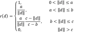
To robustify against outlier influences, M-estimators (Huber, 1964) can be applied for residual weighting. The influence of a residual (derivative of the sum of squares with respect to ) for the unweighted case is ‖ ‖. M-estimators apply a weighting function to the residuals which modifies the influence to follow a specified design. We choose the Hampel estimator (Hampel, 1986) which is a redescending variant (10).
=
{
, < ‖ ‖ ≤
‖ ‖ , < ‖ ‖ ≤
‖ ‖ − ‖ ‖− , < ‖ ‖ ≤ , ‖ ‖ >
(10)
It separates the space of absolute residuals into four sections, using three thresholds , , . Residuals below remain unweighted. The influence of residuals is fixed at for values between and and linearly scaled down to zero for values between and . Finally, the influence is eliminated for values
larger . We reset the thresholds in every iteration as follows: is set to the current standard deviation � of the unweighted residuals, is set to � and to max ‖ ‖ . Effectively we only use the first three sections of the estimator. In our experience, full suppression of outlier candidates may be corruptive in first iterations. However, the redescending characteristic of the third section usually proves helpful.
Furthermore, we put a permanent lower boundary of one pixel to and enforce ≤ ≤ . This may result in convergence and fusion of the boundaries. In cases of fusion of b and c, the resulting estimator corresponds to the Huber estimator. If all thresholds reach equality, the result corresponds to a completely unweighted case. Figure 2 illustrates the adaptive weighting scheme. The weighting function is applied to the objective function as a diagonal weighting matrix �.
Figure 2. Illustration of residual weighting using Hampel estimator. Top: first iteration, bottom: after first outlier removal. The histogram of residuals (black) is overlaid with the weighting function (solid green) and corresponding influence function (solid red). The vertical dashed lines indicate the barriers , and (from left to right). Histogram and influence function are scaled for clarification.
4.2 Numerical Stabilization through Column Equilibration
Variables whose derivatives differ widely in magnitude may cause numerical instability during matrix inversions. In our case, introduction of the distortion parameters makes it necessary to take corresponding counter measures. For this purpose, we apply column equilibration (Demmel, 1997) to precondition the Jacobian. It may be interpreted as a normalization of variable space and is applied to the Jacobian as a weighting of unknowns. We compute a normalization factor for every unknown and apply it as a diagonal matrix �. The least squares equation is modified to:
��− � = − (11)
In practice, the Jacobian is equilibrated and the adjustment is carried out as usual, which corresponds to solving for �− � . Accordingly, the correct solution is found by left hand multiplication with E. For better readability in the following section, we substitute � = ̃. The solution update � with residual weightings finally reads:
� = � ̃′� ̃− ̃′� − (12)
The reciprocal RMS of each column’s non-zero entries is used as factor for the corresponding unknowns. In order to reduce the influence of outliers, we do not compute the factors directly from the Jacobian, but from its weighted pendant, i.e. � . We have tested other variants and visually compared the resulting surface reconstructions regarding completeness and noise level. While differences were negligible in most cases, this variant performed notably best on some datasets.
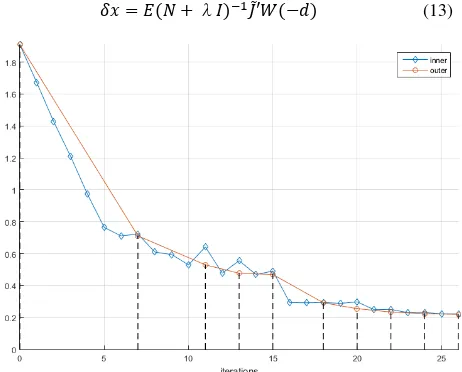
4.3 Levenberg-Marquardt with Step Size Control
To achieve robustness against weak starting values we choose to use the Levenberg-Marquardt (LM) approach. Here, we apply a simple step size control to avoid unnecessary recomputation of the Jacobian . In basic LM, every solution � of a Gauß-Newton (GN) step (outer loop) is checked for whether it actually improves the residuals. If this is the case, the starting solution is updated and the next GN step is triggered. If not the case, the solution is damped and shifted towards a steepest gradient solution by emphasizing the diagonal of the normal matrix � = ̃′� ̃ by increasing a damping factor λ.
� = � � +λ − ̃′� − (13)
Figure 3. Plot of convergence behavior. Residuals are plotted against inner iterations (blue). The dashed vertical lines and orange curve indicate nine outer iterations. After the fourth outer iteration the full camera model is applied, causing a stronger improvement. Outlier removal is triggered after the sixth outer iteration.
This is repeated (damping inner loop) until an improvement is achieved and a new GN step can be triggered. In both cases, on a successful test, the damping factor is decreased. The Jacobian is only recomputed within the outer loop. We modify the approach by an additional accelerating variant of the inner loop. I.e. on success we decrease the damping factor, update our solution and recompute the residuals as well as the weights, but keep the current Jacobian. We iterate with the fixed Jacobian until a failure occurs. In some cases the inner loop
shows convergent behavior, causing ineffective iterations. As a counter measure we terminate the inner loop when its convergence falls below 1%. After termination, the next GN step is started and a full update is computed. This results in an adaptive acceleration of convergence in steeper regions of the solution landscape. An example is given in Figure 3, where in total 26 inner iterations, whose main workload lies in the recomputation of , are needed. The much more expensive recomputation of the Jacobian is carried out only nine times within the outer GN loop.
4.4 Successive Camera Calibration and Outlier Removal
As additional intrinsic camera parameters to camera constant (focal length) and principal point, we choose radial ( , , ) and tangential (�, � ) distortions as defined in the Brown model (Brown, 1966). With �̃, being image point coordinates w.r.t. the principal point and � being the corresponding distance, ∆� is composed as the sum of:
Δ�� = (�̃
�̃ ) � + � + �6 (14)
Δ�� = � � + �̃ + � �̃ �̃
� (� + �̃ ) + � �̃ �̃ (15)
Aspect and skew could be added either within ∆� (Brown parameters � , �) or the camera matrix K, but we neglect these parameters, since usually they are insignificant. Note that the distortions are applied to the observations in order to fit to the idealized model, whereas usually in BA the idealized projection of a point is corrected to fit to the observation. If needed, e.g. to compute undistorted images, the parameters can be inverted in a separate estimation.
Due to high correlations, weak camera constellations can cause drifting or erratic convergence behavior for the intrinsic camera parameters, especially in combination with weak starting values. In order to reduce this effect, we choose to start the adjustment with a reduced camera model, including only the camera constant and . We iterate until the improvement of a GN step falls below 20%, then add the principal point and, in the last step, add the remaining parameters , , � and �. When this state is reached, we trigger outlier removal with a � threshold when improvement falls below 5%. The process is stopped if improvement stays below this level for three subsequent outlier removals.
4.5 Datum Definition
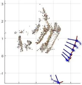
The system has a rank deficiency of order seven, which corresponds to an undefined seven parameter rigid transformation (three rotation parameters, three translations and scale). A common way to overcome this is to fix the first cameras’ position and rotation for the first six degrees of freedom. Often, one position coordinate of the second camera is fixed for overall scale. The corresponding unknowns are removed from the system (hard constraint). Alternatively, the distance between two cameras can be fixed. In cases of weak initial values for the first camera, this may lead to slow convergence behavior, especially during first iterations. In contrast, we define the datum by fixing mean position, mean rotation (sum of rotation matrices) and mean distances between cameras as additional constraint equations (weak constraints). This allows all cameras to move freely as in a geodesic free network adjustment and, if necessary, results in strong ISPRS Annals of the Photogrammetry, Remote Sensing and Spatial Information Sciences, Volume III-3, 2016
corrections to the first camera, whereas other cameras may rest in place. An example can be found in Figure 4. Here seven images are linearly distributed, with a large base between first and second image. If available, datum information from GPS, IMU, control points, scale bars etc. may be incorporated. However, our current implementation does not include these measures. non-sequential and structureless approach to SfM, which is being developed at present and outlined briefly in the following.
We extract SIFT features (Lowe, 2004) for every image and compute coarse relative orientations using a RANSAC procedure with a non-triangulating chirality test. The relative orientations are refined using the scheme described in the previous chapter. However, at this stage of our workflow we neither solve for intrinsic camera parameters, nor explicitly remove potential outliers. Weak image pairs are filtered by residuals. We apply further filtering by rotational inconsistency between triplets. The remaining triplets are then oriented by the estimation of camera poses based on the pairwise orientations. The result is refined, again using our adjustment approach. At this stage, we solve for the camera constant and to reduce drifting caused by incorrect values for these parameters. Very similar to the approach described in (Moulon et al., 2013), the triplets are used for global camera orientation. In the next step, we augment the approach by creating larger subsets based on triplet connectivity and refine these by adjustment. Again, this measure is taken to reduce drifts. Also, at this stage the adjustment is carried out as described in chapter 4, including the full camera model and outlier removal. The subsets are fused globally in the same fashion as the triplets and the result obtained by this procedure is used to initialize a final adjustment. During the whole procedure no triangulated points are used.
We evaluate the approach on the Datasets HerzJesuP8, EntryP10, FountainP11 and HerzJesuP25 of the benchmark datasets presented in (Strecha et al., 2008). The numbers in the names indicate the number of images. We omit the ‘Castle’ datasets, as our current SfM implementation produces instable results here. For the used datasets, ground truth is given for camera orientation as well as the camera matrix K. The given
images are corrected for radial (K1 and K2), but not for tangential distortion. Additionally, we have measured visible cross targets and triangulated these points using the ground truth information. We added three manually measured natural points to the datasets Entryp10 and FountainP11, since only three targets are visible.
We run our process with both suggested cost functions, but otherwise identical settings. We omit the given ground truth and initialize the focal length with the length of the image diagonal, which deviates roughly by 10% from the given value. We use the image center as initial value for principal point and initialize the distortion parameters with zero. Furthermore, we assume that all images of a dataset share the same camera model. As a reference solution, we process the datasets using PhotoScan (Version 1.1.6) with identical distortion parameters activated. The measured target points were not used within our adjustment, as this is at present not implemented. Accordingly, they remained unused for the PhotoScan orientations.
As the used camera model differs from the model used for the ground truth and to account for correlations between the estimated parameters and (subsequent) structure estimation, we evaluate in two different ways. The results given in Table 1 are obtained by registering the estimated camera stations to the ground truth positions. The transformation is estimated as a seven parameter rigid transform using unweighted least squares adjustment. We evaluate the deviations in the camera stations after transformation and compute the rotational error as geodesic distance in SO(3) (Hartley et al., 2013).
Position RMS [mm] Rotation [°] Table 1. Deviation between exterior orientation ground truth and estimated results after transformation using the camera stations (S: symmetric, A: accumulated, P: PhotoScan).
For the results in Table 2, we register using the triangulated targets (and natural points) and evaluate the differences in these points. Here, we additionally evaluate the dataset IF15D800E, which consists of 36 images of a storage/garage building in a stone quarry, captured with a Nikon D800E and a 24mm lens. No ground truth is given for the camera orientation and calibration. However, reference values, derived from laserscanning, are available for cross targets which are visible in the images. For our computations, we initialize the focal length of the dataset IF15D800E by the given approximate metric value and known pixel size.
The results indicate that in general all three variants perform comparably. The result obtained for EntryP10, processed with accumulated epipolar distances, clearly stands out as unsatisfactory. The reason is at present unclear and might as well be found within the applied SfM procedure, rather than the adjustment used therein. In general, though otherwise not clearly represented by the numerical results of this evaluation, ISPRS Annals of the Photogrammetry, Remote Sensing and Spatial Information Sciences, Volume III-3, 2016
there is a tendency for the accumulated cost function to generate stronger noise in subsequent surface reconstruction using Dense Image Matching. This circumstance is also indicated by the reprojection errors of the SIFT features, as can be seen in Table 3. Generally, the effect is stronger for datasets of lower image quality. We assume the results could be improved by incorporating the residual weighting into the functional model as a ‘root of weighted mean of squares’. A visual comparison of some results is given in Figure 6. For comparability, all surfaces are computed using SURE (Rothermel et al., 2012), by importing the corresponding camera orientations and undistorted images. The used software settings are identical.
Repro. Position RMS [mm] deviations between the corresponding 3D reference points and estimated points. The first column lists the number of targets and the mean ground sampling distance (GSD) at the targets. For the datasets EntryP10 and FountainP11, three manually measured natural points have been added to the three automatically measured targets (S: symmetric, A: accumulated, P: PhotoScan). iteration), Gauß-Newton iterations, final RMS of epipolar distances and corresponding reprojection error for the feature points.
Table 3 also lists the number of rows of the Jacobian for the suggested cost functions and the Gauß-Newton iterations required for the final adjustment. As expected, the benefit of the accumulated variant differs in terms of size reduction. The reduction is small for datasets with low redundancy, since twofold observations dominate in these cases. However, for datasets with high redundancy, e.g. HerzJesuP25 and IF15D800E, the reduction is significant. Our actual intention for
future development is to use both functional models within the adjustment to achieve further reduction. Related to convergence speed, there is no notable difference between the two costs. The listed reprojection errors are obtained by reprojection of the SIFT features after nonlinear least squares triangulation. To simulate an outlier removal of a classical bundle adjustment, we remove the worst 1% before computing the overall error.
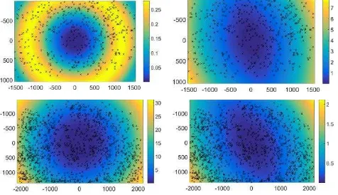
Regarding camera calibration, we do not encounter unexpected behavior. As usual, images with strong distortions or weak initial camera constant can lead to strong drifts, especially in absence of loop closure. Of course, the camera could be pre-calibrated and reference points could be used. Figure 5 illustrates exemplary distortion results. As expected, the estimated radial distortions reach maximal magnitudes of around one pixel for the Datasets of (Strecha et al., 2008).
Figure 5. Magnitude of distortion results in pixel units. Left: radial distortion; Right: tangential distortion; Top: HerzJesuP8. As expected, the remaining radial distortion is low for this dataset, since the input images have been corrected for the parameters K1 and K2. Bottom: Exemplary result for a dataset with original images.
In our experience, the additional computational workload of a scale consistency constraint may not be necessary for a wide range of image acquisition scenarios. However, if implementations aim at a general applicability, it should be taken into account. Also, our current first implementations show improved stability and convergence behavior for the triplet phase of our SfM procedure.
6. SUMMARY & OUTLOOK
We have shown that camera calibration with distortion parameters can be incorporated to structureless bundle adjustment and results with precision in object space comparable to standard bundle adjustment can be obtained. To our knowledge this has not been verified in practice before. We have developed a robustified procedure which incorporates Levenberg-Marquardt with step size control and usually converges in a reasonable number of Gauß-Newton steps. We suggested two variants of cost functions which reduce the number of equations and demonstrated experimentally that both can be applied successfully - though with different quality at present. Since integration of scale consistency constraints is needed for general applicability, we will also continue developments in this direction, while following the concept of constraint accumulation.
Figure 6. Meshed surfaces with normal shading. Datasets from left to right: HerzJesuP25, FountainP11 and IF15D800E. In top down order: symmetric cost function, accumulated cost function, PhotoScan. The corresponding orientation data and undistorted images have been used to reconstruct the surfaces with SURE, using identical settings. While differences are marginal in general, the accumulated cost function produces higher noise in some cases, as can be seen at the example of HerzJesuP25.
REFERENCES
Brown, Duane C., 1966. Decentering distortion of lenses.
Photometric Engineering 32(3), pp. 444-462.
Demmel, J. W., 1997. Applied numerical linear algebra. Siam, p. 62
Hampel, F. R., Ronchetti, E. M., Rousseeuw, P. J., & Stahel, W. A., 1986. Robust statistics: the approach based on influence functions (Vol. 114). John Wiley & Sons.
Hartley, R., 1998. Minimizing Algebraic Error in Geometric Estimation Problem. Proceedings of Sixth International Conference on Computer Vision.
Hartley, R., Trumpf, J., Dai, Y., Li, H., 2013. Rotation averaging. International journal of computer vision, 103(3), pp. 267-305.
Huber, Peter J., 1964. Robust estimation of a location parameter. The Annals of Mathematical Statistics 35(1), pp. 73-101.
Indelman, V., 2012. Bundle adjustment without iterative structure estimation and its application to navigation. Position Location and Navigation Symposium (PLANS), 2012 IEEE/ION.
Indelman, V., Roberts, R., Beall, C., Dellaert, F., 2012. Incremental light bundle adjustment. Proceedings of the British Machine Vision Conference (BMVC 2012), pp. 3-7.
Lowe, D. G., 2004. Distinctive Image Features from Scale-Invariant Keypoints. International Journal of Computer Vision, 60, 2, pp. 91-110.
Moulon, P., Monasse, P., Marlet, R., 2013. Global fusion of relative motions for robust, accurate and scalable structure from motion. In Proceedings of the IEEE International Conference on Computer Vision, pp. 3248-3255.
Rodriguez, A. L., López-de-Teruel, P. E., A. Ruiz, 2011a. Reduced epipolar cost for accelerated incremental SfM.
Computer Vision and Pattern Recognition (CVPR), 2011 IEEE Conference on.
Rodriguez, A. L., López-de-Teruel, P. E., A. Ruiz, 2011b. GEA Optimization for live structureless motion estimation. Computer Vision and Pattern Recognition (CVPR), 2011 IEEE Conference on.
Rothermel, M., Wenzel, K., Fritsch, D., Haala, N., 2012. Sure: Photogrammetric surface reconstruction from imagery. In
Proceedings LC3D Workshop, Berlin, pp. 1-9.
Steffen, R., Frahm J.-M., Förstner W., 2010. Relative bundle adjustment based on trifocal constraints. Trends and Topics in Computer Vision. Springer Berlin Heidelberg, 2012. pp. 282-295.
Strecha, C., von Hansen, W., Gool, L. V., Fua, P., Thoennessen, U., 2008. On benchmarking camera calibration and multi-view stereo for high resolution imagery. Computer Vision and Pattern Recognition (CVPR), 2008 IEEE Conference on.
Triggs, B., McLauchlan, P. F., Hartley, R. I., Fitzgibbon, A. W., 2000. Bundle adjustment—a modern synthesis. In Vision algorithms: theory and practice. Springer Berlin Heidelberg. pp. 298-372.