MLPNP - A REAL-TIME MAXIMUM LIKELIHOOD SOLUTION TO THE
PERSPECTIVE-N-POINT PROBLEM
S. Urban, J.Leitloff, S.Hinz
Institute of Photogrammetry and Remote Sensing, Karlsruhe Institute of Technology Karlsruhe Englerstr. 7, 76131 Karlsruhe, Germany - (steffen.urban, jens.leitloff, stefan.hinz)@kit.edu
http://www.ipf.kit.edu
Commission III, WG III/1
KEY WORDS:pose estimation, perspective-n-point, computer vision, photogrammetry, maximum-likelihood estimation
ABSTRACT:
In this paper, a statistically optimal solution to the Perspective-n-Point (PnP) problem is presented. Many solutions to the PnP problem are geometrically optimal, but do not consider the uncertainties of the observations. In addition, it would be desirable to have an internal estimation of the accuracy of the estimated rotation and translation parameters of the camera pose. Thus, we propose a novel maximum likelihood solution to the PnP problem, that incorporates image observation uncertainties and remains real-time capable at the same time. Further, the presented method is general, as is works with 3D direction vectors instead of 2D image points and is thus able to cope with arbitrary central camera models. This is achieved by projecting (and thus reducing) the covariance matrices of the observations to the corresponding vector tangent space.
1. INTRODUCTION
The goal of the PnP problem is to determine the absolute pose (rotation and translation) of a calibrated camera in a world refer-ence frame, given known 3D points and corresponding 2D image observations. The research on PnP has a long history in both the computer vision and the photogrammetry community (here called camera or space resectioning). Hence, we would first like to emphasize the differences between the definitions used in both communities.
PnP Classically in literature, basically two definitions of the problem exist (Hu and Wu, 2002). In the first, thedistance based definition, the problem is formulated in terms of the distances from the projective center to each 3D points, e.g. leading to min-imal P3P solutions (Haralick et al., 1991). The second definition istransformation based. Here, the task is to determine the 3D rigid body transformation between object-centered and camera centered coordinate systems, e.g. (Fiore, 2001, Horaud et al., 1989). In both PnP definitions, however, the camera is always as-sumed to be calibrated and known, allowing to transform image measurements into unit vectors, that point from the camera to the 3D scene points. More recent approaches extend this classical definition by including unknown camera parameters into the for-mulation such as the focal length (Wu, 2015) or radial distortion (Kukelova et al., 2013).
Camera resectioning The task in the photogrammetric defini-tion of the problem is to find the projecdefini-tion matrixλu=P3×4X that transforms homogeneous 3D scene points X to homoge-neous 2D image pointsu(Hartley and Zisserman, 2003, Luh-mann et al., 2006). The projection matrix is given byP3×4 = K[R|t]and hence contains the camera matrixKas well as the rotationRand translationt.
Thus, fundamentally, the main difference between the definitions in both communities is, that PnP solves only for the absolute pose of the same, calibrated camera. In camera resectioning the cam-era is assumed to be unknown and thus part of the formulation of the problem. In this paper, we assume the camera to be calibrated
and known, thus we present a solution to the Perspective-n-Point problem.
Still, the need for efficient and accurate solutions is driven by a large number of applications. They range from localization of robots and object manipulation (Choi and Christensen, 2012, Collet et al., 2009), to augmented reality (M¨uller et al., 2013) implementations running on mobile devices and having only lim-ited resources, thus focusing on fast solutions. Especially in in-dustry, surveying or medical environments, involving machine vision, (close-range) photogrammetry (Luhmann et al., 2006), point-cloud registration (Weinmann et al., 2011) and surgical nav-igation (Yang et al., 2015), methods are demanded, that are not only robust, but also return a measure of reliability.
Even though the research on the PnP problem has a long history, few work has been published on efficient real-time solutions, that take the observation uncertainty into account. Most algorithms focus on geometric but not statistic optimality. To the best of our knowledge, the only work, that includes observation uncertainty into their framework is the Covariant EPPnP of Ferraz et al. (Fer-raz et al., 2014a).
In this paper, we propose a novel formulation of a Maximum Likelihood (ML) solution to the PnP problem. Further, a gen-eral method for variance propagation from image observations to bearing vectors is exploited to avoid singular covariance matri-ces. In addition, we benchmark our real-time method against the state-of-the-art and show on a ground truth tracking data set, how our statistical framework can be used, to get a measure of the ac-curacy of the unknowns given the knowledge about the uncertain observations.
2. RELATED WORK
points are (Kneip et al., 2011),(Li and Xu, 2011) and (DeMenthon and Davis, 1992). The stability of such algorithms under noisy measurements is limited, hence they are predominately employed in RANSAC (Fischler and Bolles, 1981) based outlier rejection schemes. Apart from the P3P methods, the P4P (Fischler and Bolles, 1981, Triggs, 1999) and P5P (Triggs, 1999) algorithms exist, still dependent on a fixed number of points.
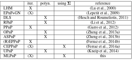
Most solvers, however, can cope with an arbitrary number of fea-ture correspondences. Basically, they can be categorized into iter-ative, non-iterative or polynomial, non-polynomial solvers. Table 1 lists all methods that are in addition evaluated in the experimen-tal section.
Iterative solutions use different objective functions, that are min-imized. In case of LHM (Lu et al., 2000) the pose is initial-ized using a weak perspective assumption. Then they proceed by iteratively minimizing the object space error, i.e. orthogo-nal deviations between observed ray directions and the corre-sponding object points in the camera frame. In the Procrustes PnP (Garro et al., 2012), the error between the object and the back-projected image points is minimized. The back-projection is based on the iteratively estimated transformation parameters. As iterative methods usually are only guaranteed to find local minima, (Schweighofer and Pinz, 2008) reformulated the PnP problem into a semidefinite programme (SDP). Despite its O(n) complexity, the runtime of the global optimization method re-mains tremendous.
Likewise, early non-iterative solvers were computational demand-ing, especially for large point sets. Among them (Ansar and Daniilidis, 2003) with O(n8
), (Quan and Lan, 1999) with O(n5 ) and (Fiore, 2001) with O(n2
). The first efficient non-iterative O(n) solution is the EPnP by (Moreno-Noguer et al., 2007), that was subsequently extended by (Lepetit et al., 2009), employing a fast iterative method to improve the accuracy. The efficiency comes from the reduction of the PnP problem to finding the po-sition of four control points that are a weighted sum of all 3D points. After obtaining a linear solution, the weights of the four control points is refined using Gauss-Newton optimization.
The most recent, non-iterative state-of-the-art solutions are all polynomial solvers: The Robust PnP (RPnP) (Li et al., 2012) first splits the PnP problem into multiple P3P problems, that re-sult in a set of fourth order polynomials. Then the squared sum of those polynomials as well as its derivative is calculated and the four stationary points are obtained. The final solution is selected as the stationary point with the smallest reprojection error. In the Direct-Least-Squares (DLS) (Hesch and Roumeliotis, 2011) method, a nonlinear object space cost function is formulated and polynomial resultant techniques are used to recover the (up to 27) stationary points of a polynomial equation system of fourth order polynomials. A drawback of this method is the parametrization of the rotation in the cost function by means of the Cayley param-eters. To overcome this, the Accurate and Scalable PnP (ASPnP) (Zheng et al., 2013b) and the Optimal PnP (OPnP) (Zheng et al., 2013a) use quaternion based representation of the rotation ma-trix. Subsequently, the (up to 40) solutions are found using the Gr¨obner basis technique on the optimality conditions of the alge-braic cost function.
The linear, non-iterative Unified PnP (UPnP) (Kneip et al., 2014) goes one step further and integrates the solution to the NPnP (Non-Perspective-N-Point) problem. The DLS formulation is ex-tended to include non-central camera rays and the stationary points of the first order optimality conditions on the sum of object space errors are found using the Gr¨obner basis methodology.
Thus far, all methods assume, that the observations are equally accurate and free of erroneous correspondences. The first PnP method, that includes an algebraic outlier rejection scheme within the pose estimation, is an extension of the EPnP algorithm called Robust Efficient Procrustes PnP (REPPnP) (Ferraz et al., 2014b). Outliers are removed from the data by sequentially eliminating correspondences that exceed a threshold on an algebraic error. The procedure remains efficient, as the algorithm operates on the linear system, spanned by the virtual control points of EPnP and thus avoids recalculating the full projection equation in each iter-ation. After removing the outliers, the final solution is attained by iteratively solving the closed-form Orthogonal Procrustes prob-lem.
Yet another extension to the aforementioned EPPnP is termed Co-variant EPPnP (CEPPnP) (Ferraz et al., 2014a). It is the first algorithm to inherently incorporate observation uncertainty into the framework. Again the linear control point system of EPnP is formulated. Then the covariance information of the feature points is transformed to that space using its Jacobian. Finally, the Maximum Likelihood (ML) minimization is approximated by an unconstrained Sampson error.
In this paper, we propose a new real-time capable, statistically optimal solution to the PnP problem leveraging observation un-certainties. We propagate 2D image uncertainties to general bear-ing vectors and show, how a linear ML solution with non-sbear-ingular covariance matrices can be obtained by using the reduced obser-vation space presented by F¨orstner (F¨orstner, 2010). In contrast to the CEEPnP, where the ML estimator is used, to obtain an es-timation of the control point subspace, we optimize directly over the unknown quantities, i.e. rotation and translation and thus, di-rectly obtain pose uncertainties. Finally, we compare the results of our algorithm to a ground truth trajectory and show, that the estimated pose uncertainties are very close to the ground-truth.
iter. polyn. usingΣ reference
LHM X (Lu et al., 2000)
EPnP+GN (X) (Lepetit et al., 2009)
DLS X (Hesch and Roumeliotis, 2011)
RPnP X (Li et al., 2012)
PPnP X (Garro et al., 2012)
OPnP X (Zheng et al., 2013a)
ASPnP X (Zheng et al., 2013b)
(R)EPPnP X (Ferraz et al., 2014b)
CEPPnP (X) X (Ferraz et al., 2014a)
UPnP X (Kneip et al., 2014)
MLPnP (X) X this
Table 1. Comparison of all tested methods. The methods are categorized into being iterative or a polynomial solver and if they incorporate measurement uncertaintyΣ. (X) depicts methods, that refine a preliminary result iteratively.
3. MLPNP
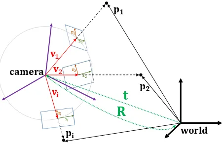
The task of Perspective-n-Point (PnP) is to find the orientation R∈SO(3)and translationt∈R3that maps theIworld points pi, i= 1, .., Ito their corresponding observationsviin the
cam-era frame. This relation is given by:
λivi=Rpi+t (1)
whereλiare the depths of each point and the observationsviare
the measured and thus uncertain quantity having unit length, i.e. kvik= 1. In the following the methodology of our algorithm is
�
Figure 1. Observations of object points from a camera. The planes at each bearing vector vi are spanned by its respective
null space vectorsriandsi.
3.1 Observations and uncertainty propagation
Let a world pointpi ∈ R
3
be observed by a calibrated camera and let the uncertain observation in the image plane be:
x′
where the uncertainty about the observed point is described by the 2D covariance matrixΣx′x′. Assuming an arbitrary interior orientation parametrization, the image pointx′
is projected to its corresponding three dimensional direction in the camera frame, using the forward projection functionπ(e.g. K−1
in the
per-withJπbeing the Jacobian of the forward projection. Thus, the
uncertainty of the image pointx′
is propagated using:
where the rank of the covariance matrixΣxx is two, i.e. it is singular and not invertible. Subsequent spherical normalization yields the final and general observation. We will refer to them as bearing vectors:
following (F¨orstner, 2010) the covariance is propagated using:
Σvv=JΣxxJ
Observe, that the covariance matrixΣvvremains singular, i.e. a Maximum Likelihood (ML) estimation based on the three resid-ual components of bearing vectors is invalid. Thus, a minimal representation of the covariance information for the redundant representation of the homogeneous vectorvis desirable. In the following section, we will introduce the nullspace of vectors and show how this can be subsequently used to get an initial estimate
of the absolute orientation of the camera.
3.2 Nullspace of bearing vectors
The following was developed by (F¨orstner, 2010). The nullspace ofv, spans a two dimensional coordinate system whose axis, de-noted as rand s, are perpendicular tov and lie in its tangent space:
The functionnull(·)calculates the Singular Value Decomposi-tion (SVD) ofv and takes the two eigenvectors corresponding to the two zero eigenvalues. Further we assumeJvr to be an orthonormal matrix, i.e. JTvr(v)Jvr(v) = I2. Note, thatJvr in addition represents the Jacobian of the transformation from the tangent space to the original vector. Thus the transposeJT
vr
yields the transformation from the original homogeneous vector vto its reduced equivalentvr.
vr=
Another way to think aboutvr is as a residual in the tangent
space. In the following, we will exploit Eq. 8 to get a linear estimate of the rotation and translation of the camera in the world frame by minimizing this residual in the tangent space.
3.3 Linear estimation of the camera pose
Using Eq.1 and 7 we can reformulate Eq. 8:
camera, the projection of a world pointpi to the tangent space
of v, should result in the same reduced coordinates, i.e. zero residual. Expanding Eq. 10 yields:
0 =r1(ˆr11px+ ˆr12py+ ˆr13pz+ ˆt1)
unknowns, i.e. we can stack them in a design matrixAto obtain a homogeneous system of linear equations:
Au=0 (12)
observa-tions, the stochastic model is given by:
P=
Σ−1
v1
rv
1
r . . . 0
..
. . .. ... 0 . . . Σ−1
vi
rvir
(13)
and the final normal equations are:
ATPAu=Nu=0 (14)
We find theuthat minimizes Eq. 14 subject tokuk= 1, using SVD:
N=UDVT (15)
The solution is the particular column ofVthat corresponds to the smallest singular value inD:
ˆ R=
ˆ
r11 rˆ12 rˆ13 ˆ
r21 rˆ22 rˆ23 ˆ
r31 r32 r33
,t= ˆ
t1,ˆt2,ˆt3
(16)
It is determined up to a scale factor, thus the translational part ˆ
tonly points in the right direction. The scale can be recovered from the fact, that the norm of each columnˆr1,ˆr2andˆr3of the rotation matrixRˆ must equal one. Hence, the final translation is:
t= p3 ˆt
kˆr1kkˆr2kkˆr3k (17)
The exploited constrain shows, that the 9 rotation parameters do not define a correct rotation matrix. This, can be solved by calcu-lating the SVD ofRˆ:
ˆ
R=URDRVRT (18)
and the best rotation matrix minimizing the Frobenius norm is found as:
R=URVTR. (19)
Up to this point, a linear ML estimation of the absolute camera pose is obtained. To increase the accuracy, a non-linear refine-ment procedure is used. Doing a subsequent refinerefine-ment of the initial estimate is a common procedure, e.g. performed in (Lep-etit et al., 2009), (Ferraz et al., 2014b) or (Lu et al., 2000).
3.4 Non-linear refinement
We apply a Gauss-Newton optimization to iteratively refine the camera pose. Specifically, we minimize the tangent space resid-uals defined in Eq. 10. This is reasonably fast for two reasons. On the one hand, the nullspace vectors are already calculated and we simply have to calculate the dot products between the tangent space vectors and each transformed world point. On the other hand, the results of the linear estimates are already close to a local minimum, i.e. the Gauss-Newton optimization converges quickly. In practice we found, that a maximum number of five iterations is sufficient. To arrive at a minimal representation of the rotation matrix, we chose to expressRin terms of the Cayley parametrization (Cayley, 1846).
3.5 Planar case
In the planar case, the SVD (Eq.15) yields up to four solution vectors, as the corresponding singular values become small (close to zero). In this case, the solution is a linear combination of those vectors. To solve for the coefficients, an equation system with non-linear constraints had to be solved. We avoid this using the following trick. LetM= [p1,p2, ..,pi]be a 3×Imatrix of all
world points. The eigenvalues ofS=MMTgive us information
about the distribution of the world points. In the ordinary 3D case, the rank of matrixSis three and the smallest eigenvalue is not close to zero. In the planar case, the smallest eigenvalue becomes small and the rank of matrixSis two. If the world points lie on a plane that is spanned by two coordinate axis, respectively, i.e. one of the elements of all world points is a constant, we could simply omit the corresponding column from matrixAand get a distinct solution.
In general, the points can lie on an arbitrary plane in the world frame. Thus, we use the eigenvectors ofSas a rotation matrix RSand rotate the world points to a new frame using:
ˆ
pi=RTSpi (20)
Here, we can identify the constant element of the coordinates and omit the corresponding column from the design matrixA. Note, that this transformation does not change the structure of the prob-lem. The rotation matrix obtained after SVD (Eq. 19), simply has to be rotated back to the original coordinate frame:
R=RSR (21)
To keep our method as general as possible, the matrixSis always calculated. We then simply switch between the planar and the or-dinary case, depending on the rank of the matrixS. To determine the rank we use rank-revealing QR decomposition with full piv-oting and set a threshold (1e-10) on the smallest eigenvalue.
4. RESULTS
In this section, we compare our algorithm to all state-of-the-art algorithms using synthetic as well as real data. To reasonably assess the runtime performance of each algorithm, we categorize the state-of-the-art solvers according to their implementation:
Matlab
OPnP (Zheng et al., 2013a), EPPnP (Ferraz et al., 2014b), CEPPnP (Ferraz et al., 2014a), DLS (Hesch and Roumelio-tis, 2011),
LHM (Lu et al., 2000), ASPnP (Zheng et al., 2013b), SDP (Schweighofer and Pinz, 2008), RPnP (Li et al., 2012), PPnP (Garro et al., 2012)
C++,mex
UPnP (Kneip et al., 2014), EPnP+GN (Lepetit et al., 2009), MLPnP (this paper)
Note however, that the Matlab implementations of many algo-rithms are already quite optimized, and it is unclear how large the performance increase of a C++ version would be.
Our method is implemented in both Matlab and C++. We in-tegrated the C++ version in OpenGV (Kneip and Furgale, 2014). The Matlab version will be made publicly available from the web-site of the corresponding author, i.e. all results are reproducible. All experiments have been conducted on a Laptop with Intel Core [email protected].
4.1 Synthetic experiments
toolbox and are briefly described in the following. All experi-ments are repeatedT = 250times and the mean pose errors are reported.
Assume a virtual calibrated camera with a focal length off = 800 pixels. First, 3D points are randomly sampled in the camera frame on the interval [-2, 2]×[-2, 2]×[4,8] and projected to the image plane. Then, the image plane coordinatesx′
are perturbed by Gaussian noise with different standard deviationsσyielding a covariance matrix Σx′x′ for each feature. At this point, we arrived at Eq. 2.
Now, the image plane coordinatesx′
are usually transformed to normalized image plane coordinates applying the forward projec-tionπ. In the synthetic experiment, this simplifies to perspective division:x = [x′
/f, y′ /f,1]T
. Most algorithms work with the first two elements ofx, i.e. normalized image plane coordinates. Instead, we apply Eq. 5 and spherically normalize the vectors, to simulate a general camera model. Further, we propagate the covariance information using Eq. 6.
Finally, the ground truth translation vectortgt is chosen as the
centroid of the 3D points and the ground truth rotationRgt is
randomly sampled. Subsequently, all points are transformed to the world frame yieldingpi.
The rotation accuracy in degree betweenRgtandRis measured
asmax3
k=1(arccos(r
T
k,gt·rk)×180/π), whererk,gtandrare
the k-th column of the respective rotation matrix. The translation accuracy is computed in % asktgt−tk/ktk ×100.
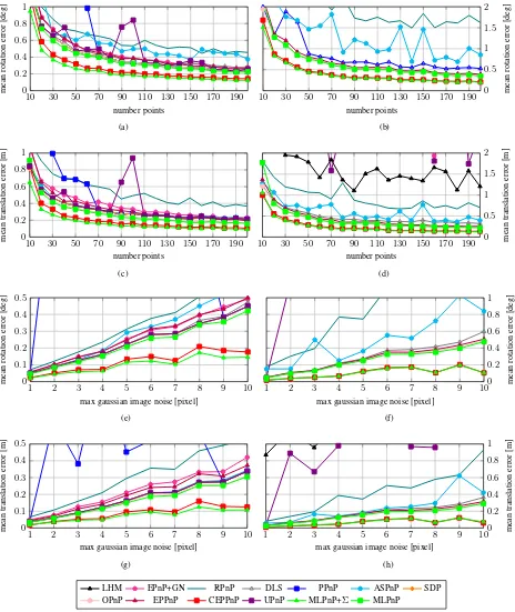
The first column of 3 depicts the ordinary and the second column the planar case, where theZcoordinate of the world points is set to zero. The first two rows of Fig. 3 depict the mean accuracy for rotation and translation for an increasing number of points (I=10,..,200). Following the experiments of (Ferraz et al., 2014a), the image plane coordinates are perturbed by Gaussians withσ= [1,..,10] and 10% of the features are perturbed by each noise level, respectively.
For the third and fourth row of Fig. 3 the number of features is kept constant (I=50) and only the noise level is increased. This time, a randomσis chosen for each feature from 0 to the maxi-mum number, ranging from 0 to 10.
The experiments for the ordinary case show, that MLPnP outper-forms all other state-of-the-art algorithms in terms of accuracy. Moreover, it stays among the fastest algorithms as depicted in Fig. 2. For less than 20 points, the algorithm is even faster than EPnP, that is still the fastest PnP solution.
4.2 Real Data
To evaluate the performance of our proposed MLPnP method on real data, we recorded a trajectory of T = 200 poses of a mov-ing, head mounted fisheye camera in an indoor environment. The camera is part of a helmet multi-camera system depicted in Fig. 4a. We use the camera model of (Scaramuzza et al., 2006) and the toolbox of (Urban et al., 2015) to calibrate the camera. All sensors have a resolution of 754×480 pixels and are equipped with equal fisheye lenses. The field of view of each lens cov-ers185◦
. The ground truth posesMtgtare obtained by a Leica
T-Probe, mounted onto the helmet and tracked by a Leica laser-tracker. This tracker was in addition used to measure the 3D coor-dinates of the world points. The position accuracy of this system isσpos≈100µm= 0.1mmand the angle accuracy is indicated
withσangle≈0.05mrad.
(a) (b)
Figure 4. (a) Camera system with mounted T-Probe. The back-ground shows the lasertracker. (b) Some images taken from the trajectory. Tracked world points are depicted in green.
For each frametin the trajectory, the epicenters ofIpasspoints (planar, black filled circles) are tracked over time, as depicted in Fig. 4b. The number of passpoints I, that are visible in each frame ranges from 6 to 13.
To assess the quality of the estimated camera pose, we calculate the mean standard deviation (SD)σ¯Randσ¯tof the relative orien-tation between camera and T-Probe. The relative orienorien-tation for each frame is calculated as follows:
Mrel=M
−1
gtMt (22)
whereMt = [R,t]is the current camera pose and is estimated
by each of the 13 algorithms respectively.
4.3 Including Covariance Information
For the first framet = 1, the covariance information about the measurementsΣx′x′ is set to the identityI2for each feature. To this point, the only thing we know about the features is, that they are measured with identical accuracy of 1 pixel. For the following framet= 2, however, estimation theory can tell us, how well a point was measured in the previous frame, given the estimated parameter vector.
LetAbe the Jacobian of our residual function Eq. 10. Then, the covariance matrix of the unknown rotation and translation param-eters is:
Σˆrˆt= (A T
PA)−1
(23)
and cofactor matrix of the observations:
Qvrvr =AΣˆrˆtA T
(24)
Observe, that this gives us the cofactor matrix in the reduces ob-servation space. Thus, we project them back to the true observa-tion space of the respective point i:
Σvivi=Jvi
r(vi)QvirvirJ
T
vi
r(vi) (25)
10 500 1
,000 1,500 2,000
0 50 100 150 200 250
number points
ex
ecution
time
[ms]
(a)
10 500 1
,000 1,500 2,000
0 5 10 15 20
number points
ex
ecution
time
[ms]
(b)
LHM EPnP+GN RPnP DLS PPnP ASPnP SDP
OPnP EPPnP CEPPnP UPnP MLPnP+Σ MLPnP
Figure 2. Runtime. (a) All methods. (b) Zoom to the fastest methods. CEPPnP and MLPnP+Σincorporate measurement uncertainty. All other algorithms assume equally well measured image points.
4.4 External vs. internal accuracies
Usually, it is desirable to have a measure of reliability about the result of an algorithm. A common approach in geometric vision, is to quantify the quality of the pose in terms of the reprojection error. Most of the time, this might be sufficient. Many com-puter vision systems are based on geometric algorithms and need a measure of how accurate and robust objects are mapped in the camera images. But sometimes it is useful to get more infor-mation about the quality of the estimated camera pose, e.g. for probabilistic SLAM systems. As MLPnP is a full ML estimator, we can employ estimation theory to obtain the covariance infor-mation about the estimated pose parameters and thus their stan-dard deviations as a measure of reliability. Letrbe the vector of stacked residuals[dri, dsi]T. First, we calculate the variance
factor:
σ2 0=
rTPr
b (26)
withPbeing the stochastic model andb= 2I−6is the redun-dancy of our problem. Then, the 6×6 covariance matrixΣˆrˆtof the unknowns is extracted with Eq. 23. Finally, the 6×1 vector of standard deviations of the camera pose is:
σˆr,ˆt=σ0
p
diag(Σˆrˆt) (27)
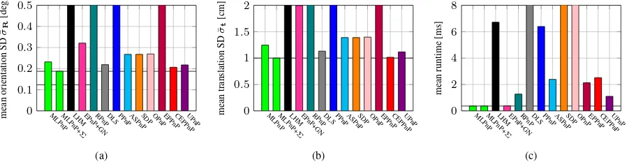
We extract the covariance matrix for every frame in the trajectory and calculate the mean standard deviation over all frames. Tab. 2 depicts the results compared to the standard deviation that was calculated to the ground truth. The marginal differences between the internal uncertainty estimations and the external ground truth uncertainties is an empirical proof that our proposed ML estima-tor is statistically optimal.
σangle[deg] σpos[cm]
ground truth 0.19 1.03
estimated 0.18 0.92
Table 2. Comparison between the estimated (internal) uncertainty and the uncertainty obtained by the ground truth (external)
5. CONCLUSION
In this paper, we proposed a Maximum Likelihood solution to the PnP problem. First, the variance propagation from 2D image
observations to general 3D bearing vectors was introduced. The singularity of the resulting 3×3 covariance matrices of such bear-ing vectors motivated the subsequent reduction of the covariance to the vector tangent space. In addition, this reduced formula-tion allows to obtain a soluformula-tion to the PnP problem in terms of a linear Maximum Likelihood estimation followed by a fast iter-ative Gauss-Newton refinement. Finally the method was tested and evaluated against all state-of-the-art PnP methods. It shows similar execution times compared to the fastest methods and out-performs the state-of-the-art in terms of accuracy.
ACKNOWLEDGMENT
This project was partially funded by the DFG research group FG 1546 ”Computer-Aided Collaborative Subway Track Planning in Multi-Scale 3D City and Building Models”. In addition the au-thors would like to thank Patrick Erik Bradley for helpful discus-sions and insights.
REFERENCES
Ansar, A. and Daniilidis, K., 2003. Linear pose estimation from points or lines. IEEE Transactions on Pattern Analysis and Ma-chine Intelligence (PAMI) 25(5), pp. 578–589.
Cayley, A., 1846. About the algebraic structure of the orthogonal group and the other classical groups in a field of characteristic zero or a prime characteristic. Reine Angewandte Mathematik. Choi, C. and Christensen, H. I., 2012. Robust 3D visual tracking using particle filtering on the special euclidean group: A com-bined approach of keypoint and edge features. International Jour-nal of Robotics Research (IJRR) 31(4), pp. 498–519.
Collet, A., Berenson, D., Srinivasa, S. S. and Ferguson, D., 2009. Object recognition and full pose registration from a single image for robotic manipulation. In: Proceedings of the IEEE Interna-tional Conference on Robotics and Automation (ICRA), pp. 48– 55.
DeMenthon, D. and Davis, L. S., 1992. Exact and approximate solutions of the perspective-three-point problem. IEEE Trans-actions on Pattern Analysis and Machine Intelligence (PAMI) 14(11), pp. 1100–1105.
Ferraz, L., Binefa, X. and Moreno-Noguer, F., 2014a. Leveraging feature uncertainty in the PnP problem. In: Proceedings of the British Machine Vision Conference (BMVC).
10 30 50 70 90 110 130 150 170 190 0
0.2
0
.4
0
.6
0.8
1
number points
mean
rotation
error
[de
g]
(a)
10 30 50 70 90 110 130 150 170 190
0 0 .5 1 1 .5 2
number points
mean
rotation
error
[de
g]
(b)
10 30 50 70 90 110 130 150 170 190
0 0
.2
0.4
0 .6 0
.8 1
number points
mean
translation
error
[m]
(c)
10 30 50 70 90 110 130 150 170 190
0 0
.5
1 1
.5
2
number points
mean
translation
error
[m]
(d)
1 2 3 4 5 6 7 8 9 10
0 0
.1
0
.2
0
.3
0.4
0
.5
max gaussian image noise [pixel]
mean
rotation
error
[de
g]
(e)
1 2 3 4 5 6 7 8 9 10
0 0 .2 0
.4 0
.6
0.8
1
max gaussian image noise [pixel]
mean
rotation
error
[de
g]
(f)
1 2 3 4 5 6 7 8 9 10
0 0
.1 0
.2 0
.3 0
.4 0
.5
max gaussian image noise [pixel]
mean
translation
error
[m]
(g)
1 2 3 4 5 6 7 8 9 10
0 0 .2 0
.4 0
.6 0
.8 1
max gaussian image noise [pixel]
mean
translation
error
[m]
(h)
LHM EPnP+GN RPnP DLS PPnP ASPnP SDP
OPnP EPPnP CEPPnP UPnP MLPnP+Σ MLPnP
MLPnPMLPnP+
Σ
LHMEPnP+GNRPnPDLS PPnP ASPnPSDP OPnPEPPnPCEPPnPUPnP
0
LHMEPnP+GNRPnPDLS PPnP ASPnPSDP OPnPEPPnPCEPPnPUPnP
0
LHMEPnP+GNRPnPDLS PPnP ASPnPSDP OPnPEPPnPCEPPnPUPnP
0
Figure 5. (a) mean orientation and (b) mean translation standard deviation over all frames of the real trajectory. (c) mean runtime over all frames. CEPPnP and MLPnP+Σincorporate measurement uncertainty. All other algorithms assume equally well measured image points.
Fiore, P. D., 2001. Efficient linear solution of exterior orientation. IEEE Transactions on Pattern Analysis and Machine Intelligence (PAMI) 23(2), pp. 140–148.
Fischler, M. A. and Bolles, R. C., 1981. Random sample consen-sus: a paradigm for model fitting with applications to image anal-ysis and automated cartography. Communications of the ACM 24(6), pp. 381–395.
F¨orstner, W., 2010. Minimal representations for uncertainty and estimation in projective spaces. In: Proceedings of the Asian Conference on Computer Vision (ACCV), Springer, pp. 619–632. Garro, V., Crosilla, F. and Fusiello, A., 2012. Solving the PnP problem with anisotropic orthogonal procrustes analysis. In: Sec-ond International Conference on 3D Imaging, Modeling, Process-ing, Visualization & Transmission, pp. 262–269.
Haralick, R. M., Lee, D., Ottenburg, K. and Nolle, M., 1991. Analysis and solutions of the three point perspective pose esti-mation problem. In: Proceedings of the IEEE Conference on Computer Vision and Pattern Recognition (CVPR), pp. 592–598. Hartley, R. and Zisserman, A., 2003. Multiple view geometry in computer vision. Cambridge University Press, New York, NY, USA.
Hesch, J. A. and Roumeliotis, S. I., 2011. A direct least-squares (DLS) method for PnP. In: Proceedings of the International Con-ference on Computer Vision (ICCV), pp. 383–390.
Horaud, R., Conio, B., Leboulleux, O. and Lacolle, L. B., 1989. An analytic solution for the perspective 4-point problem. In: Pro-ceedings of the IEEE Conference on Computer Vision and Pattern Recognition (CVPR), pp. 500–507.
Hu, Z. and Wu, F., 2002. A note on the number of solutions of the noncoplanar P4P problem. IEEE Transactions on Pattern Analysis and Machine Intelligence (PAMI) 24(4), pp. 550–555. Kneip, L. and Furgale, P., 2014. OpenGV: A unified and gen-eralized approach to real-time calibrated geometric vision. In: Proceedings of the IEEE International Conference on Robotics and Automation (ICRA), pp. 1–8.
Kneip, L., Li, H. and Seo, Y., 2014. UPnP: An optimal O(n) solution to the absolute pose problem with universal applicability. In: Proceedings of the European Conference on Computer Vision (ECCV), Springer, pp. 127–142.
Kneip, L., Scaramuzza, D. and Siegwart, R., 2011. A novel parametrization of the perspective-three-point problem for a di-rect computation of absolute camera position and orientation. In: Proceedings of the IEEE Conference on Computer Vision and Pattern Recognition (CVPR), pp. 2969–2976.
Kukelova, Z., Bujnak, M. and Pajdla, T., 2013. Real-time solution to the absolute pose problem with unknown radial distortion and focal length. In: Proceedings of the International Conference on Computer Vision (ICCV), pp. 2816–2823.
Lepetit, V., Moreno-Noguer, F. and Fua, P., 2009. EPnP: An accurate O(n) solution to the PnP problem. International Journal of Computer Vision (IJCV) 81(2), pp. 155–166.
Li, S. and Xu, C., 2011. A stable direct solution of perspective-three-point problem. International Journal of Pattern Recognition in Artificial Intelligence 25(05), pp. 627–642.
Li, S., Xu, C. and Xie, M., 2012. A robust O(n) solution to the perspective-n-point problem. IEEE Transactions on Pattern Anal-ysis and Machine Intelligence (PAMI) 34(7), pp. 1444–1450. Lu, C.-P., Hager, G. D. and Mjolsness, E., 2000. Fast and glob-ally convergent pose estimation from video images. IEEE Trans-actions on Pattern Analysis and Machine Intelligence (PAMI) 22(6), pp. 610–622.
Luhmann, T., Robson, S., Kyle, S. and Harley, I., 2006. Close range photogrammetry: Principles, methods and applications. Whittles Publishing. Dunbeath, Scotland.
Moreno-Noguer, F., Lepetit, V. and Fua, P., 2007. Accurate non-iterative O(n) solution to the PnP problem. In: Proceedings of the International Conference on Computer Vision (ICCV), pp. 1–8. M¨uller, M., Rassweiler, M.-C., Klein, J., Seitel, A., Gondan, M., Baumhauer, M., Teber, D., Rassweiler, J. J., Meinzer, H.-P. and Maier-Hein, L., 2013. Mobile augmented reality for computer-assisted percutaneous nephrolithotomy. International journal of computer assisted radiology and surgery 8(4), pp. 663–675. Quan, L. and Lan, Z., 1999. Linear n-point camera pose deter-mination. IEEE Transactions on Pattern Analysis and Machine Intelligence (PAMI) 21(8), pp. 774–780.
Scaramuzza, D., Martinelli, A. and Siegwart, R., 2006. A flexi-ble technique for accurate omnidirectional camera calibration and structure from motion. In: Proceedings of the Fourth IEEE Inter-national Conference on Computer Vision Systems (ICVS, pp. 45– 45.
Schweighofer, G. and Pinz, A., 2008. Globally optimal O(n) solu-tion to the PnP problem for general camera models. In: Proceed-ings of the British Machine Vision Conference (BMVC), pp. 1– 10.
Triggs, B., 1999. Camera pose and calibration from 4 or 5 known 3D points. In: Proceedings of the International Conference on Computer Vision (ICCV), Vol. 1, pp. 278–284.
Urban, S., Leitloff, J. and Hinz, S., 2015. Improved wide-angle, fisheye and omnidirectional camera calibration. ISPRS Journal of Photogrammetry and Remote Sensing 108, pp. 72–79. Weinmann, M., Weinmann, M., Hinz, S. and Jutzi, B., 2011. Fast and automatic image-based registration of TLS data. ISPRS Jour-nal of Photogrammetry and Remote Sensing 66(6), pp. S62–S70. Wu, C., 2015. P3.5P: Pose estimation with unknown focal length. In: Proceedings of the IEEE Conference on Computer Vision and Pattern Recognition (CVPR), pp. 2440–2448.
Yang, L., Wang, J., Ando, T., Kubota, A., Yamashita, H., Sakuma, I., Chiba, T. and Kobayashi, E., 2015. Vision-based endoscope tracking for 3D ultrasound image-guided surgical navigation. Computerized Medical Imaging and Graphics 40, pp. 205–216.
Zheng, Y., Kuang, Y., Sugimoto, S., Astrom, K. and Okutomi, M., 2013a. Revisiting the PnP problem: A fast, general and opti-mal solution. In: Proceedings of the International Conference on Computer Vision (ICCV), pp. 2344–2351.