FINE REGISTRATION OF KILO-STATION NETWORKS - A MODERN PROCEDURE
FOR TERRESTRIAL LASER SCANNING DATA SETS
J.-F. Hullo a*
a Electricité De France Lab Paris-Saclay - 7 boulevard Gaspard Monge, 91120 Palaiseau. [email protected]
Commission V, WG V/3
KEY WORDS: Registration, Terrestrial laser scanners, 3D-Network, Graph, Spectral analysis ABSTRACT:
We propose a complete methodology for the fine registration and referencing of kilo-station networks of terrestrial laser scanner data currently used for many valuable purposes such as 3D built reconstruction of Building Information Models (BIM) or industrial as-built mock-ups. This comprehensive target-based process aims to achieve the global tolerance below a few centimetres across a 3D network including more than 1,000 laser stations spread over 10 floors. This procedure is particularly valuable for 3D networks of indoor congested environments. In situ, the use of terrestrial laser scanners, the layout of the targets and the set-up of a topographic control network should comply with the expert methods specific to surveyors. Using parametric and reduced Gauss-Helmert models, the network is expressed as a set of functional constraints with a related stochastic model. During the post-processing phase inspired by geodesy methods, a robust cost function is minimised. At the scale of such a data set, the complexity of the 3D network is beyond comprehension. The surveyor, even an expert, must be supported, in his analysis, by digital and visual indicators. In addition to the standard indicators used for the adjustment methods, including Baarda’s reliability, we introduce spectral analysis tools of graph theory for identifying different types of errors or a lack of robustness of the system as well as in fine documenting the quality of the registration.
Figure 1: front view of the kilo-stations network of the TLS dataset of a cylindrical industrial building. On the left, concrete walls and floors of the buildings, with a human silhouette for scale. The sights of all targets as seen from TLS stations are traced in blue; TLS stations (one thousand) are the reds dots and control points are the larger green spheres.
1. INTRODUCTION
From cultural heritage to industrial purposes, the use of 3D as-built mock-ups has become a standard for many applications. To maintain facilities for instance, the knowledge of 3D geometry of the factory is valuable through many use-cases: maintenance planning, handling, storage, replacement or replacement of important components.
Such as-built 3D models (CAD or BIM format) are reconstructed (or adjusted) as close as possible to a 3D point cloud, acquired in situ in compliance with the quality requirements (exhaustiveness, accuracy, precisions and reliability). This cloud is thus considered as a reliable source to describe the geometry of the facility in its current state.
Indoor point clouds are generally produced by using a laser scanner which scans the entire scene with a laser. For one point of view, the current laser scanners can measure in less than
10 minutes a point cloud including 40 million points with a 5 mm tolerance on most objects (not too dark, nor too reflective, at less than 30 m). Then as many points of view as necessary are performed to remove masks and cover the entire area under study: in an indoor and congested environment, 1 station is provided on average every 10 to 15 m² to remove the major part of the masks. For an entire building with several floors, hundreds of scans can be achieved rapidly. In the case of the reactor building of a nuclear power plant, for instance, which contains 10 circular floors of 60 m in diameter, there are more than 1,000 laser scan stations.
Nevertheless, due to the pair-pair registration error propagation, the assembly errors of these independent scans rapidly become preponderant in recordings of this size. Unfortunately, in complex indoor scenes, not only is there no GNSS to estimate poses, but the inter-visibilities between the targets and stations are weak and therefore restrict the robustness of the network.
This paper describes a global adjustment method for kilo-station networks recommended and implemented for large indoor laser scan networks. The aim of this method is to allow and warrant compliance with the quality requirements (precision, accuracy and reliability) on large scan networks. This paper specifically contributes to this purpose through the following:
Reduced formalisation (Gauss-Helmert) of the target-based registration problem.
Review of the main cost functions and discussion concerning the loss algorithms.
Global scheme for the analysis of large 3D networks, especially with graph analysis tools for laser station networks (spectral analysis and algebraic connectivity). Proposals concerning methods for identifying
“outliers” (gross errors) at the level of the constraints between the stations.
The whole article is illustrated by experiments carried out on real data sets, including a network of 1,000 laser stations
2. STATE OF THE ART
A 3D cloud point is a set of � coordinates ��(��, ��, ��), calculated in the case of an acquisition by laser scanner from measurements of a horizontal angle ��, a vertical angle �� and a direct distance ��. It is agreed that we are to write ��� the point whose coordinates are expressed in the coordinate system ��. The uncertainty on the final point cloud is modelled (approximation) at each point for a variance-covariance 3ൈ3 matrix Σ�� . This variance-covariance matrix contains all of the error components of the acquisition process (Reshetyuk, 2009). Firstly, the polar observations are marred by instrumental and environmental measurement errors (Lichti, 2007). The shape of the object (angle of incidence, edge effects, reflectance, etc.) also modifies the laser signal on the distance measurement. These errors on the observations can then be expressed by error propagation in a Cartesian format. Finally, the referencing uncertainty on these data in an external coordinate system, whether it is related to another station or global, also influences the final coordinates (Reshetyuk, 2009).
The change in coordinate system �� to ��, which is used to express several scans in the same system, is referred to as registration when system �� is an arbitrary system of one of the measuring and referencing when ��= �� is a pre-existing global system (�: �����). Many methodologies have been developed to solve the registration of the point cloud. The cloud-to-cloud approaches directly use the point cloud to establish the constraints used in the pose estimation (Rusinkiewicz and Levoy, 2001) and (Pomerleau et al., 2013). The approaches per targets use higher level features extracted in the point cloud (point in the centre of a sphere, cylinder reconstructed on a pipe, floor drawing, etc.) generally solved according to the least squares criterion (Rabbani, 2006) and (Hullo et al., 2011). In the case of recordings of cluttered indoor scenes, cloud-to-cloud methods are difficult to use for topographical purposes, both due to their high calculation consumption rate and to their lack of robustness. For the registration such as for the referencing of large networks, the judicious arrangement of targets in the environment remains a very productive method for ensuring the centimetric accuracy ranges (Hullo et al., 2015). Cloud-to-cloud constraints can nevertheless still be implemented in case of a failed use of the targets (manual segmentation of connected sub-clouds or refinement steps between station pairs). This refining stage is often used to improve the final results (Gelfand et al., 2005).
In the case of large networks of internal laser stations, the registration problems can therefore be expressed as a problem concerning the adjustment of the constraints between targets recognised from several points of view. It is this analogy of this problem with the geodetic networks that has been exploited in the past for referencing methods referred to as “direct” and which use traversing survey methods (Lichti, Gordon and Tipdecho, 2005). However, for large scan networks (exceeding 100 stations), a block calculation using the least squares method, such as proposed in (Mikhail, 1976) or more recently in (Strang and Borre, 1997), is generally implemented such as in the network of 500 stations in a cave (Gallay et al., 2015).
Yet, such as pointed out in (Scaioni, 2012), the use of common tools in geodesy is hardly referred to in literature concerning the registration of large laser networks, which become the daily work of a certain number of surveyors. For a long time, geodesy has tackled the adjustment of large measurement networks (Helmert, Cholesky, Bowie, etc.) and (Golub and Plemmons, 1980). (Meissl, 1980) provides the orders of magnitude of the American datum consisting of ~ 350,000 unknowns (~ 170,000 stations) and ~ 2 million observations; in comparison, one thousand laser scans consists of ~ 6,000 unknown ~ and 30,000 constraints (3 per target). The introduction of reliability concepts by (Baarda, 1968) has provided new additional analysis tools for Geodesists which are used, for instance, for internal networks (tunnels) (Gründig and Bahndorf, 1984). Furthermore, the use of influence functions adapted to various error models, tolerating a percentage of non-Gaussian errors (Huber, 1964) and (Hampel et al., 1986), has been implemented during the development of fuzzy statistics in geodesy (Carosio and Kutterer, 2001), of probabilistic methods such as processed by (Koch, 1990) and of the analysis of the deformation of large networks (Caspary, 2000). (Triggs et al., 2000) refers back to all of the block-based adjustment methods by describing various formulations and cost functions and by underlining the significance of the use of effective methods for minimising sparse sets of linear algebra systems (Ashkenazi, 1971). (Agarwal, Burgard and Stachniss, 2014) offers an initial cross reading between the geodetic methods and the Graph-SLAM (Simultaneous Localization and Mapping).
It is also through the formalism of the Graph-SLAM that the strong connection between the adjustment of 3D networks and the graphs is revealed (Olson, 2008). While linear algebra is often used for the adjustment of 3D networks, the graph theory was not exploited initially in the various work concerning the optimisation and design of geometric networks (Grafarend, 1985) and (Kuang, 1991). Only a few uses have been identified: in (Tsouros, 1980), (Katambi and Jiming, 2002) and (Theiler, Wegner and Schindler, 2015). Therefore, many tools can be used for understanding and analysing a measurement network (graph) (Berge, 1958). These numerical analysis tools are especially useful when, such as in the case of a 3D network comprising hundreds of stations spread over many floors, the visual representation of the latter is too complex to be easily analysed. The spectral graph theory is one of the most powerful tools for these topological analysis. It focuses on the eigenvalues and eigenvectors of the adjacency or Laplacian matrices of the graphs (Brouwer and Willem, 2011). The meaning to be given to these spectra has been studied for many physical problems (Tinkler, 1972), road problems (Maas, 1985) or even cognitive science problems (de Lange, de Reus and van den Heuvel, 2014). Some uses for GNSS networks were also proposed (Even-Tzur, 2001), (Katambi and Jiming, 2002), (Lannes and Gratton, 2009) and (Even-Tzur and Nawatha, 2016).
3. MODELLING TLS AND TARGETS NETWORKS 3.1 Variables
A laser scanner performs, from one point of view, an overview referred to as “station”. The coordinates of point ��� in �� and those of point ��� in �� are connected, in general, by:
��=
� �
��. �� �+ �� � (1)
⎣ ⎢⎢ ⎡������
�� � ⎦⎥⎥
⎤= ��(���). ��(���). ��(���).
⎣ ⎢⎢ ⎡���
�� �
�� �
⎦ ⎥⎥ ⎤
+ ⎣ ⎢⎢ ⎡������
�� � ⎦⎥⎥
⎤
Where ( �0� , �0� , �0)� are the coordinates in system �� of centre �� of the station; (���, ���, ���) are the Cardan angles of rotation matrices ���� and �� around respective axes �⃗ �⃗ and �⃗. It is considered that the corrections of systematic errors on angular observations were made during the transition from polar to Cartesian.
Thanks to the internal bi-axial compensator of some laser scanners, we can consider two other transformation models. The vertical model considers the value of angles ���= ���= 0 as insignificant. The model can be simplified (4 settings) but can generate significant registration errors if verticality has not been fully ensured during the acquisition phase. The near-vertical model gives way to small variations of these angles, either through the addition of linear terms, or for an increased robustness through the addition of pseudo-constraints with the following value ���= ���= 0 and variances ��2 and ��2 provided by calibrating the biaxial compensator.
3.2 Constraints and weights
A target seen from at least two stations creates a geometric constraint between these two stations (Hullo et al., 2011). Among the various geometric primitives that can be used to identify constraints, we favour the use of point features extracted from targets arranged for this purpose in the environment (centre of a sphere or chequered target). The surface properties (sphericity, reflectance, etc.) of the targets shall be analysed (Wunderlich et al., 2013).
3.3 Target matching
The correct creation of this set of constraints directly conditions the quality of the registration results due to the fact that, in the case of non-robust methods (least squares), a single matching error directly impacts the calculation results. This is all the more significant in the case of large laser networks where the probability of a matching error and the difficulty related to the identification of these faults increase with combinatorics. Hence, finding the best set of correspondences is a combinatorial optimisation problem with an acceptance assumption. Although the simplest solution is performing a comprehensive search, it becomes rapidly impossible to perform. Three approaches are generally employed: the search tree methods (Vosselman, 1995), the pose clustering methods (Olson, 1997) or the RANSAC-type stochastic method proposed in (Rabbani and van den Heuvel, 2005) for primitive-based registration of laser scans.
In all cases, reducing the search space is not only required to reduce the calculation time, but it also reduces the probability of mismatches if the reduction criteria make sense and if the search
subset makes sense. In order to constrain the search, it is necessary to define relevant features (Rabbani, 2006). Firstly, selecting a neighbouring station involves using as an a priori approximate values of the stations, obtained by indoor positioning such as described in (Hullo et al., 2012). The viability of a configuration is then tested by an initial RANSAC matching process, which is performed in three steps, such as described in (Rabbani, 2006) with, as a similarity distance, the probabilistic score defined in (Hullo et al., 2012), which is used to decide the matches selected from the a priori of the stations and targets.
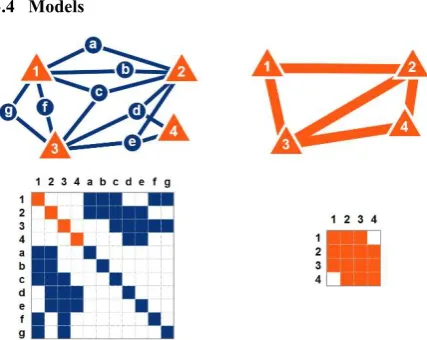
3.4 Models
Figure 2: diagram and normal equations associated to parametric (left) and Gauss-Helmert (right) models
Figure 3: top view of a target-stations 3D sub-network plot (110 stations) with parametric (left) and Gauss-Helmert (right) models
In a parametric adjustment model, the constraint created by the matching � ≡ � of a sphere view from two stations �� and �� is:
��
� = ���� . ( ��� − ��)� ��
� = �
��� . ( ��� − ��)�
The match � ≡ � indicates that ���= ��� . This observation equation amounts to expressing observations as a function of the unknown values, or otherwise to "simulating" the observations � with the unknown values :
�(�) = �
�(�0) + �. �� = �� where � =���� (2) A variance-covariance matrix is used to weight the observations. Through the linearisation of the constraint equations close to the approximate values of the parameters, we can write a system of normal equations corresponding to type �� = �, which can be solved by many well-known methods in linear algebra (Strang and Borre, 1997). But this parametric formulation requires calculating the coordinates of the spheres as unknown values, which significantly complicates the calculations. However, this
formulation allows one to analyse the contributions of the matched targets in the calculation one by one.
Another formulation, which can be considered as reduced, is to directly consider the constraint matching:
���. ��� + ��� = ���. ���� + ���
This mixed method, referred to as the Gauss-Helmert method (Mikhail, 1976), is to express a condition directly linking observations and unknown values as follows:
�(�, �) = 0 �(�0, �0) + �. �� + �. �� = 0
With � =���� and � =����
(3)
The advantage of this formulation is the reduction of the problem, both for viewing and for solving the calculation.
3.5 Acquisition and structure
The acquisition stage of both laser data and control network surveying should comply with the expert methods specific to surveyors. For registering laser scans, each station should reasonably see in average 8 targets and every pair of consecutive stations should share in average 5 targets (without weak configurations). For referencing targets on tie network, we recommend at least 5 targets per independent network and an average of 1 control target for 4 laser stations.
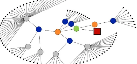
Figure 4: tree-structure of a hundred laser scans (black) registered consecutively in sub-networks (grey > blue > orange > green), up to referencing to external coordinate system using control points (red square)
These tie points can be integrated either as fixed conditions or pseudo-observations, to which are associated variances, also called soft constraints (Strang and Borre, 1997). This second option offers more flexibility in large-scale calculations. Moreover, the models also allow the integration of topographic measurements (angles and distances) into the same calculation. This integration is not recommended due to the summary of independent error budgets between surveying and lasergrammetry, but it can be used to locally complete a weak control network.
Independent blocks of stations can be created freely in situ. If they are completely independent and if the support points are known with an accuracy of a greater order of magnitude, they can be referenced through an affine transformation. However, a total block adjustment provides a better control of the referencing network which can, at least during an intermediate calculation phase, be relevant. The use of sub-blocks can then be used through the calculations to facilitate the resolution (Bjerhammar, 1973). By means of error propagation, we recommen not to exceed a sub-block nesting level greater than 3.
4. SOLVING REGISTRATION 4.1 Cost function
The least squares, which minimise a quadratic form of the residues, are an unbiased estimator of a linear regression for variables according to a normal distribution (Mikhail, 1976). When functions connecting observations and unknown values are not linear, the loss/minimisation process is iterative (Bjerhammar, 1973) and (Mikhail, 1976).
However, the data sets are often marred by gross errors which deviate from the Gaussian model and can significantly influence the results. These outliers must be removed from the data set because the quadratic function increases the influence of important residuals. These outliers are generally detected via statistical tests. However, the latter fail if the proportion of outliers becomes too high (Huber, 2009). It is then necessary to adopt a new model with reasonable errors, which involves a related cost function (Koch, 2007) that makes the influence of the residues consistent with the error model.
(�|�) ∝ ∏ �(��|�)�
�=1 → max
− ln �(�|�) ∝ ∑ − ln �(��|�)�
�=1 → min
(4)
�(��) = − ln �(��|�) is introduced as the general functional of M-estimators. The MAP assessment is thus defined in the case of independent observations by:
∑ ���� �(��)
�=1 → min
(5)
In case the observations are not completely independent, (Bjerhammar, 1973) has shown that a multidimensional variable (residues), which follows a normal distribution law, can always be transformed into a reduced and centred multidimensional variable. This basic change is performed upstream of the adjustment thanks to the following relationship:
�~�(�, Σ) ⇔ � ∶= Σ1/2 � + � �ℎ��� � ~�(0, �) (6)
In (Triggs et al., 2000), the functional is defined as �(����), which does not make it possible to process the outliers that are summed prior to the application of the functional. (Yang, Song and Xu, 2002) offers functional �(�)���(�) which finally generalises the functional of equation (5) for many loss functions (Zhang, 1997). In the case of laser networks and due to the number of observations and rate of errors in target matching, the Welsch functional is a great robust estimator that allows to highlight outliers.
4.2 Minimization
Since we are interested in minimising non-linear functions, precautions shall also be taken. In the case of linear least squares, the system to be solved by inversion (in actual fact, we will never directly inverse the matrix of normal equations) (Triggs et al., 2000). In the case of non-linear least squares, we will proceed by iteration on the linearisation of the functional model. However, in the case of non-linear M-estimators, it is also necessary to nest the linearisation of the cost function in the iterations. To perform these minimisations, (Triggs et al., 2000) discusses the use of the Newton and quasi-Newton methods.
In the case of large lasergrammetric networks, one thousand stations are considered, at each of which around ten targets are measured with many connections with neighbours. The global equation system is therefore large and non-linear.
Hopefully, the network structure induces sparse matrices which offer interesting possibilities in the optimisation process (Ashkenazi, 1971). In order to take advantage of digitally efficient methods, it is advisable to rely, at a minimum, on effective linear algebra libraries (LAPACK type) or on libraries dedicated to statistical regression methods (sparseLM or SBA type). Many wrappers exist for scripted languages, recommended for the development phases (Python, R, or Matlab).
5. NETWORK ANALYSIS 5.1 Principles of evaluation
The delivery of a laser data set must meet a well-defined need. This need is specified geometrically with accuracy, precision and reliability criteria, which are subject to a quality control which may be demanding, for example, in the industry where centimetric precisions at the scale of a building can be required (Hullo et al., 2015). In order to ensure these criteria as well as to allow the detection and investigation of defects, it is necessary to use relevant indicators and to establish a set of checks throughout the data production process.
However, the laser data arrives at the end of a long chain, in which each link has its own sources and types of errors. Considering the complexity of the acquisition process, the volume of data and the importance attached to the optimisation of the pose parameter assessments, it is necessary to conduct the assessment phase as an investigation, aiming to validate the quality criteria one after another: a vision which only involves considering the final indicators, without returning to their origin, is not sufficient in our case to confidently qualify the dataset.
5.2 Model assessment
Firstly, it should be ensured that the functional models (matched targets) and stochastic models (distributions/cost function and related magnitudes) are suitable for the observations used in the calculation.
Extraction of the targets - the target extraction process must produce a quality criterion, which can be used to complete matrix ���= 1
�02�� where �0
2 is an arbitrary function called an a priori
variance factor. The analysis of this matrix is to help identify suspicious targets and guide the inspection work.
Matching - this is a key aspect in the adjustment process. Matching is a decision (Boolean) to establish a correspondence between two targets acquired from different stations and the analysis of these errors is different from a fault detection on a scalar value. The search for matching errors is processed separately at the end of this section. Checks on the number of correspondences between pairs of stations and the number of the target connected to the general survey marker must also be carried out in batch mode to direct the subsequent identification for gross errors.
Verticality and calibration - it is possible that the assumption retained for the condition equations is false for some stations. In a vertical or near-vertical model, we will search for major local closures �� after adjustment for all targets of a station that might have been inclined. Moreover, we will compare the standard closures ���
�� between the devices by serial number and by work sessions to detect any potential uncalibration of the instruments.
���= Σ��= �0′2. ���
where ���= ������− ������ (7)
The a posteriori variance is provided by �0′2= √��.�.�� where r is the redundancy. The ratio between the a priori and a posteriori variances indicates the consistency of the model with respect to the indicated a priori. We have the same probabilistic thresholds due to the fact that these variables follow the following law �2
�0′2 �02 ≤ ��
2
� (8)
Closures in control points - checks shall be inspected, i.e. not included as constraints in the adjustment calculation for both registration and referencing. We will specify the maximum value and the average of these deviations in relation to the checks ��. Only these checks qualify the accuracy of the final result.
Error propagation through the model - after calculation, we can assess the stochastic properties of the estimated unknown values and observations adjusted by propagation of a priori errors through the adjustment model.
Σ��= �0′2. �−1
with � = ��. (�. ���. ��)−1� (9)
In order to analyse these large variance-covariance matrices, it is a standard practise to resort to error ellipsoids which, if they only correspond to a partial representation of a large size distribution, can be used to observe unfavourable conditions for the error propagation. These propagated variances and covariances are used to assess the accuracy of the hypothesis and observations. However, the non-linearity of the functional model requires other indicators to determine the reliability of these results.
5.3 Network configuration
At the scale of a building, the complexity of the 3D network is beyond comprehension. The surveyor, even an expert, must be supported, in his analysis, by digital and visual indicators that will help him target his sampling inspection, detect quality faults and in fine qualify the data set.
Redundancy - the local redundancy �� of an observation (Karup, 2006) is defined between 0 and 1 such that a redundancy equal to 0 corresponds to an unchecked observation, which is therefore essential, and a redundancy equal to 1 corresponds to a checked observation, which therefore is useless. The sum of the local redundancies is equal to the total redundancy � = ∑ ����=1 ; �� is the ��ℎ term of the matrix diagonal ����.
Smallest gross errors (or "grossest" small errors) - a tolerance is generally defined by a probabilistic threshold (3�, 95%, etc.). Nevertheless, it is interesting to know, for each observation, the limit value for undetectable gross errors ∇��, referred to as internal reliability (Baarda, 1968). For this purpose, we set � the type II error probability (false negative) and ���� the fault threshold, which can be used to calculate the translation parameter �. Internal reliabilities are given by:
∇��= �. √���
�� (10)
Sensitivity to gross errors - the external reliability, or fault simulation, is used to estimate the influences at the level of each unknown value of the smallest undetectable fault at the level of each observation (Baarda, 1968). These influences are calculated for each observation:
∇��= max� (∇���) with:
(11)
⎣ ⎢ ⎢ ⎢ ⎢ ⎡∇∇��2��1
⋮ ∇���
⋮ ∇���⎦⎥
⎥ ⎥ ⎥ ⎤
= �−1. ��. �. ⎣ ⎢⎢ ⎢ ⎡ 0⋮
∇�� ⋮ 0 ⎦
⎥⎥ ⎥ ⎤
(12)
At each point, we therefore have � vectors [∇�, ∇�, ∇�]. 2D (Baarda, 1968) proposes a rectangle defined by the vector with the largest norm (half of the long side of the rectangle) and the maximum of the norm of vectors projected perpendicularly to the first vector (half of the short side of the rectangle). We believe it is more interesting to visualise the influence of all external reliabilities. Indeed, from a user interface perspective, it seems useful to use this reliability indicator as a rake to weave a link between the unknown values and observations at the origin of these sensitivities.
Figure 5: top: rakes of reliability of a 3D network; bottom: location of the 3D network: at the top of the building, only accessible through ladders. The blue line is the sight of a referencing target; all red lines are the influence of the gross error threshold on this specific observation; this kind of interaction is helpful in the stage of outlier detection and dataset documentation.
5.4 Graph analysis
Valence analysis - In the parametric model, unique pseudo-observations created as constraints between stations are used to express the measurement network as a non-directed weighted graph, which can be expressed as a matrix either via its adjacency matrix � or its Laplacian matrix (normalized) � = � − �−1� where � is the valence matrix (degree) (de Lange, de Reus and van den Heuvel, 2014). Based on this graph, we then have a remarkable set of tools to understand the "topological" configuration of our network. Low valences nodes can be seen as bridges or parts of a weak traverse in the graph.
Spectral analysis - The spectral analysis of a graph focuses on analysing the eigenvalues �� and eigen vectors �� of the graph matrices. T. Krarup had, in the 70s, studied the spectrum of geodetic networks through eigen values of ��� (Karup, 2006). (de Lange, de Reus and van den Heuvel, 2014) explain general meanings of the Laplacian spectrum: each eigenvector �� describes a network bisection by assigning a positive or negative value to each node (the components of the eigenvector) and the associated eigenvalue describes the reverse of the division time in a stationary state. The eigenvector �1 related to the largest
eigenvalue �1 of the adjacency matrix, referred to as spectral radius or algebraic connectivity, arranges the nodes of the graph according to their centrality in the network (Maas, 1985). The �1variation upon addition or deletion of the nodes makes this eigenvalue a good indicator of the network global connectivity (de Lange, de Reus and van den Heuvel, 2014). The smallest non-zero eigenvalue ��−1 provides information on the best possible sections of the network in two modules. A possible number of subgroups for an optimum division may be suggested by the largest interval between two eigenvalues (��+1− ��). The presence of zero components in the eigenvectors of the graph also indicates the presence of independence between the sub-graphs. Each spectrum of eigenvalues therefore describes a network topology, and these topologies can be compared (Wilson and Zhu, 2008).
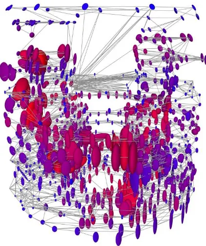
The algebraic connectivity appeared as a very reliable indicator for the data set shown in Figure 6. A ground truth registration data set was created through an exhaustive check of the 40 billion point cloud based on regular section every 50 cm along the 3 axis X, Y and Z leading to additions of local cloud-cloud constraints for ~1% of the dataset. We inspected correlations between real errors (gound truth poses vs block adjustment) and error ellipsoids (75%), reliability (55%) and connectivity (81%). A deeper analysis of these results may help understanding strength of each indicator.
Figure 6: algebraic connectivity (from red to blue) and error ellipsoid through error propagation in the model of a kilo-station network
5.5 Gross errors detection
The detection of gross errors mainly consists of, in the case of a laser network, searching for matching errors, which in most cases, have a major influence on the result of the adjustment. This complex task of target-based laser registration, described in section 3.3, is not included in the “traditional” geodetic networks. False negatives (unmatched targets) can generate weak areas in the network while false positives create a false constraint, which distorts the results. However, if a gross error is detected on a target in inter visibility, it is interesting to try and preserve a
maximum of constraints. In order to identify false positives, we therefore searched for 3 configurations per target clustering:
1 vs. all: a target is badly detected in a station, the other views of this target is consistent with one another: 1 constraint is deleted.
2 periods: we manage to distinguish two consistent sets of views of this target: we can split these two periods as two distinct targets.
Cause unknown: no structure is identified in the spheres: all constraints are removed for this target.
On the 100 largest gross errors of the network shown in Figure 6, only 18 had to be removed: 12 were only pairwise constraints that could not be corrected and 6 were unique observations of control targets (referencing observations only represent 2% of the dataset). On the remaining 82 gross errors, we could identify 70% of “1 vs all” configuration, 30% of “moving targets”. By preserving 82 gross errors, this approach have been a valuable tool for increasing precision with a minimum loss of redundancy.
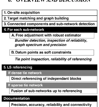
6. OVERVIEW AND DISCUSSION
Figure 7: overview of the referencing process of kilo-station networks
When solving registration, we recommend performing a calculation in several stages: free network with robust estimator (inspection of reliability, graph spectrum and precision), datum points as soft constraints (removing wrong datum points) and final least squares referencing. However, some stage still remain tedious that should first be optimized to increase productivity. The crucial stage, target matching, relies on good approximations of the poses; using coarse approximations from field sketches is always available when human performs the acquisition but fine indoor positioning systems may help. An algorithm for detecting the structure of the acquisition, for example using graph analysis tools introduced previously, may also be a valuable addition to the process. But, as so often, the user interface and interaction development might be the most valuable improvement.
7. CONCLUSION
In this paper, we described a large 3D network registration and referencing method used for blocks of hundreds of terrestrial laser scans acquired in complex internal environments whose complexity is beyond comprehension. This method, in the current state of the art of laser topographic data adjustment, uses geodetic tools for adjustment and graph theory tools for network analysis and gross error identification. In the first stage, correspondences between targets are established (adjustment and referencing). In
order to deal with the combinatorics of this problem, we propose a probabilistic method that uses a position a priori. When assembled, these constraints define a large algebraic and stochastic system which, similarly to large geodetic networks, is used to estimate the most likely pose parameters of the measurement stations. A robust functional (Welsch) is thus recommended to reduce the adjustment bias. The various accuracy, precision and reliability indicators are used to qualify the network and detect gross errors. The spectral analysis of the network, based on the breakdown into eigenvalues of the Laplacian matrix, guides the search for outliers and offers new tools for understanding these large three-dimensional networks. The target matching faults thus detected are analysed to retain a maximum of constraints while removing a maximum of false positives.
The current limitations of this method, illustrated on a real data set of a thousand stations, firstly concern the quality of the initial matching phase. To improve it, the graph theory introduced in this chapter provides real study possibilities such as spanning trees (Kirchoff's Matrix-Tree theorem) to search for faults by calculating closures or other properties of the eigenvalues to improve inspection of the network. Another issue favouring the adoption of this method to a broader audience is to develop new visualisation and interaction tools to guide the operator throughout this complex process.
ACKNOWLEDGEMENTS
The author would like to thank Emmanuel CLEDAT for its technical contributions and energy to this work.
REFERENCES
Agarwal, P., Burgard, W. and Stachniss, C. (2014) 'Survey of geodetic mapping methods: Geodetic approaches to mapping and the relationship to graph-based slam.', Robotics & Automation Magazine, IEEE, vol. 21, no. 3, pp. 63-80.
Ashkenazi, V. (1971) Geodetic normal equations in Large Sets of Linear Equations, New York: Academic.
Baarda, W. (1968) 'A testing procedure for use in geodetic networks', Netherlands Geodetic Commission: Publications on Geodesy, New Series, vol. 2, no. 5, p. 97.
Berge, C. (1958) La théorie des graphes et ses applications. , Paris: Dunod.
Bjerhammar, A. (1973) Theory of errors and generalized matrix inverses, Amsterdam.
Brouwer, A.E. and Willem, H.H. (2011) Spectra of graphs, Springer Science & Business Media.
Carosio, A. and Kutterer, H. (2001) First international symposium on robust statistics and fuzzy techniques n geodesy and GIS, Zürich: ETH.
Caspary, W.F. (2000) Concepts of network and deformation analysis, 3rd edition, Sydney: University of New South Waes. de Lange, S.C., de Reus, M.A.. and van den Heuvel, M.P. (2014) 'The Laplacian spectrum of neural networks. ', Frontiers in computational neuroscience, vol. 7, no. 1, January, pp. 1-12. Even-Tzur, G. (2001) 'Graph Theory Applications to GPS Networks', GPS Solutions, vol. 5, no. 1, July, pp. 31-38.
Even-Tzur, G. and Nawatha, M. (2016) 'Gross-Error Detection in GNSS Networks Using Spanning Trees', Journal of Surveying Engineering, January.
Gallay, M., Kanuk, J., Hochmuth, Z., Meneely, J.D., Hofierka, J. and Sedlák, V. (2015) 'Large-scale and high-resolution 3-D cave mapping by terrestrial laser scanning: a case study of the Domica
Cave, Slovakia', International Journal of Speleology, vol. 44, no. 3, September, pp. 277-291.
Gelfand, N., Mitra, N., Guibas, L. and Pottmann, H. (2005) 'Robust global registration', Eurographics Symposium on Geometry Processing, vol. 2, no. 3, July, p. 5.
Golub, G.H. and Plemmons, R.J. (1980) 'Large-scale geodetic least-squares adjustment by dissection and orthogonal decomposition', Linear Algebra and its Applications, vol. 34, March, pp. 3-28.
Grafarend, E.W. (1985) 'Criterion Matrices for Deforming Networks', in Grafarend, E.W. (ed.) Optimization and Design of Geodetic Networks, New-York: Springer.
Gründig, L. and Bahndorf, J. (1984) 'Accuracy and Reliability in Geodetic Networks—Program System Optun', J. Surv. Eng., vol. 110, no. 2, August, pp. 133-145.
Hampel, F., Ronchetti, E., Rousseeuw, P. and Stahel, W. (1986) Robust Statistics: The Approach Based on Influence Functions, New-York: John Wiley & Sons.
Huber, P.J. (1964) 'Robust estimation of a location parameter.', Ann. Math. Statist., vol. 35, no. 1, pp. 73-101.
Huber, P.J..R.E.M. (2009) Robust statistics, 2nd edition, Hoboken: John Wiley and Sons.
Hullo, J.F., Grussenmeyera, P., Landes, T. and Thibault, G. (2011) 'Georeferencing of Tls Data for Industrial Indoor Complex Scenes: Beyond Current Solutions', ISPRS-International Archives of the Photogrammetry, Remote Sensing and Spatial Information Sciences, vol. 3812, pp. 185-190. Hullo, J.F., Thibault, G., Boucheny, C., Dory, F. and Mas, A. (2015) ' Multi-Sensor As-Built Models of Complex Industrial Architectures.', Remote Sensing, vol. 7, December, pp. 16339– 16362.
Hullo, J.F., Thibault, G., Grussenmeyer, P. and Landes, T.a.B.D. (2012) 'Probabilistic feature matching applied to primitive based registration of TLS data.', ISPRS Annals Photogramm. Remote Sens., vol. 1, pp. 221-226.
Karup, T. (2006) Mathematical Foundation of geodesy, Berlin: Springer.
Katambi, S. and Jiming, G.a.W.K. (2002) 'Applications of graph theory to gross error detection for GPS geodetic control networks', Geo-spatial Information Science, vol. 5, no. 4, August, pp. 26-31.
Koch, K.R. (1990) Bayesian inference with geodetic applications, Berlin: Springer-Verlag.
Koch, K.R. (2007) Introduction to Bayesian statistics., Berlin: Springer Science & Business Media.
Kuang, S. (1991) Optimization and design of deformation monitoring schemes.
Lannes, A. and Gratton, S. (2009) 'GNSS networks in algebraic graph theory', Journal of Global Positioning Systems, vol. 8, no. 1, pp. 53-75.
Lichti, D.D. (2007) 'Error modelling, calibration and analysis of an AM–CW terrestrial laser scanner system.', ISPRS J. Photogramm. Remote Sens., vol. 61, no. 5, pp. 307-324.
Lichti, D.D., Gordon, S.J. and Tipdecho, T. (2005) 'Error models and propagation in directly georeferenced terrestrial laser scanner networks.', Error models and propagation in directly georeferenced terrestrial laser scanner networks., vol. 131, no. 4, pp. 135-142.
Maas, C. (1985) 'Computing and interpreting the adjacency spectrum of traffic networks', Journal of computational and applied mathematics, vol. 12, pp. 459-466.
Meissl, P. (1980) A priori predction of roundoff error accumulation in the solution of a super-large geodetic normal equation system, U.S. Departement of commerce.
Mikhail, E.M. (1976) Observations and least squares., New York.
Olson, C.F. (1997) 'Efficient pose clustering using a randomized algorithm', International Journal of Computer Vision, vol. 23, no. 2, pp. 131-147.
Olson, E.B. (2008) Robust and efficient robotic mapping., Cambrige: Massachusetts Institute of Technology.
Pomerleau, F., Colas, F., Siegwart, R. and Magnenat, S. (2013) 'Comparing ICP variants on real-world data sets.', Autonomous robots, vol. 34, no. 3, pp. 133-148.
Rabbani, T. (2006) Automatic reconstruction of industrial installations using point clouds and images. , Delft: NCG Nederlandse Commissie voor Geodesie Netherlands Geodetic Commission.
Rabbani, T.. and van den Heuvel, F. (2005) 'Automatic point cloud registration using constrained search for corresponding objects.', Proceedings of 7th Conference on Optical, 3-5. Reshetyuk, Y. (2009) Self-calibration and direct georeferencing in terrestrial laser scanning., Stockholm: Technology, Royal Institute of.
Rusinkiewicz, S. and Levoy, M. (2001) 'Efficient variants of the ICP algorithms', 3D Digital Imaging and Modeling.
Scaioni, M. (2012) 'On the estimation of rigid-body transformation for TLS registration.', Int. Arch. Photogramm. Remote Sens. Spatial Inf. Sci, vol. 39, no. B5.
Strang, G. and Borre, K. (1997) Linear algebra, geodesy and GPS, Wellesley-Cambridge Press edition, Wellesley.
Theiler, P.W., Wegner, J.D. and Schindler, K. (2015) 'Globally consistent registration of terrestrial laser scans via graph optimization', ISPRS J. Photogramm. Remote Sens., vol. 109, November, pp. 126-138.
Tinkler, K.J. (1972) 'The physical interpretation of eigenfuncions of dichotomous matrices.', Transactions of the Institue of British Georaphers, vol. 55, pp. 17-46.
Triggs, B., McLauchlan, P., Hartley, R. and Fitzgibbon, A. (2000) 'Bundle adjustment - a modern synthesis', ICCV '99 Proceedings of the International Workshop on Vision Algorithms: Theory and Practice, 198-372.
Tsouros, C. (1980) 'An application of graph thery to geodetic networks.', Quateriones Geodaesie, pp. 79-84.
Vosselman, G. (1995) 'Applications of tree search methods in digital photogrammetry', ISPRS J. Photogramm. Remote Sens., vol. 50, no. 4, pp. 29-37.
Wilson, R.C. and Zhu, P. (2008) 'A study of graph spectra for comparing graphs and trees.', Pattern Recognition, vol. 41, no. 9, pp. 2833-2841.
Wunderlich, T., Wasmeier, P., Ohlmann-Lauber, J., Schäfer, T. and Reidl, F. (2013) 'Objective Specifications of Terrestrial Laserscanners–A Contribution of the Geodetic Laboratory at the Technische Universität München.', Blue Series Books at the Chair of Geodesy, vol. 21, March.
Yang, Y., Song, L. and Xu, T. (2002) 'Robust estimator for correlated observations based on bifactor equivalent weights', Journal of Geodesy, vol. 76, July, p. 353+358.
Zhang, Z. (1997) 'Parameter estmation techniques: a tutorial with application to conic fitting', Image and Vision Computing, vol. 15, no. 1, January, pp. 59-76.