*Corresponding author.
E-mail address:[email protected] (P.J. Agrell).
Notation
t,i"0,2,¹ time index xt"[xt
1,2,xtm]T column vector of inputs inperiodt
x8t"[x8t1,2,x8tH]T column vector of
transform-able inputs in periodt
zJ
n"[ZI1,n,2,ZIM,n]T column vector of non-trans-formable inputs in product
nin periodt
ZI"[ZI
1,2,ZIn] matrix of non-transformableinputs in periodt
yt"[yt1,2,ytN]T column vector of outputs in
periodt
wt"[wt1,2,wtM] row vector of input prices in
periodt
w8t"[w8t1,2,w8tM] row vector of input prices in
periodt,w8t-wt
pt"[pt1,2,ptN] row vector of output prices
in periodt
A caveat on the measurement of productive e
$
ciency
Per J. Agrell
!
,
"
,
*
, B. Martin West
"
!Department of Economics, Royal Veterinary and Agricultural University, DK-1958 Frederiksberg C, Denmark
"Department of Production Economics, Linko(ping Institute of Technology, S-581 83 Linko(ping, Sweden
Received 9 April 1998; accepted 10 March 2000
Abstract
The correspondence between used performance measures and enterprise objectives, such as pro"t maximization and cost minimization, is fundamental for manufacturing companies. This paper identi"es, and critically examines, a minimal set of relevant properties that a productivity index needs to satisfy to rightly assess performance development of a decision-making unit. Commonly applied and suggested productivity measurement techniques, such as partial e$ciencies, total factor productivity (TFP), index number approaches, integrated partial e$ciencies and operational competitiveness ratings, are analyzed in order to assess the alignment with superior objectives. There is a considerable spread in the results of this class of models and the interpretation may prove di$cult or misleading. As these apparently less complicated productivity measures increasingly are employed as a component in evaluation of manufacturing e$ciency, the question is of high managerial relevance. In particular, the paper points out inconsistencies with properties related to commensurability, monotonicity, and implications of maximizing behavior. Based on this viewpoint, issues such as the consistency with pro"t maximization will be shown extra interest. The paper also provides a critique of previous work in non-parametric e$ciency analysis where properties have been postulated or based on other arguments.
The"ndings suggest that there is no globally superior measurement technique to be found in this class and that care
should be taken when evaluating managerial performance not to penalize rational behavior. ( 2001 Elsevier Science
B.V. All rights reserved.
Keywords: Productivity analysis; Performance evaluation; Total factor productivity; Index number
1. Introduction
The concept of productivity and e$ciency as
a complement to pure economic measures of performance is widely accepted in practice. Productivity, commonly expressed as a mere ratio between outputs produced and inputs consumed, is perceived as an easily interpretable measure of
op-erational performance. E$ciency denotes the
rela-tive productivity measurement resulting from a comparison with some reference, other compara-ble units and/or historical values. The outcome of the assessment of the performance of a division,
plant or unit may be further investments,
a closedown or bonuses paid to management and/or employees, prizes and other attention. It may also be indirect, such as the use of the particu-lar unit as a role model or to allocate investment budgets. In either way, it is an implicit assumption that the behavior of the decision-making unit (DMU) is coherent with organizational goals such
as pro"t maximization, shareholder wealth
maxi-mization or cost minimaxi-mization given an output level. On a grander scale, it is important for the credibility of the applied performance measure-ment technique that it is perceived as fair in an economic sense. Our viewpoint is to interpret this as not to penalize decisions that are economically sound.
However, as acknowledged in Bogetoft [1,2] and
Diewert [3], the incentive e!ects related to
well-known e$ciency measurement techniques are
am-biguous and worth further attention. Using an agency theory framework, Bogetoft [1,2] evaluates how Data Envelopment Analysis [4] measures cor-relate with rational behavior by a risk-averse agent. The author shows necessary model adjustments to
provide incentive e$cient measurements and their
sensitivity to various kinds of error and model
misspeci"cation. Diewert [3] discusses the
incen-tive e!ects of index number measurements in
regu-lated "rms. This paper is a continuation of this
stream of work in that it challenges a series of non-parametric productivity measurement tech-niques that purport to take economic issues into
account. It also extends the pro"t maximization
results presented by Caves et al. [5], Balk [6] and
FaKre and Grosskopf [7] for the Malmquist and
ToKrnqvist indexes. Eight methods are included in
the study: Total Factor Productivity indexes
Las-peyres [8], Paasche [9], Fisher [10], and ToKrnqvist
[11]; the American Productivity Center-method
[12]; the`Pro"tability"Productivity#Price
Re-coverya-method [13]; Operational Competitiveness
Ratings [14]; and Integrated Partial E$ciency [15].
This collection of measures sets out to be more readily applicable and less strenuous to calculate than other approaches, such as parametric produc-tion funcproduc-tions or frontier-based non-parametric ap-proaches, e.g. data envelopment analysis by Charnes et al. [4]. The methods in this class vary consider-ably in their structure and derivation, but all share a common data base of input and output quantities along with their prices for (at least) two periods in time and result in a scalar value for the productivity change during the period. The ratio-based methods all penalize scale and input volume in some way as
opposed to purely"nancial measures such as pro"t,
return on investment and the price/earnings ratio. Hence, there is no ambiguity about the applicabil-ity of the measures as operational alternatives to
(short-term)"nancial indicators.
The outline of the paper is straightforward, after selecting a few economically relevant properties the methods are expressed in a common notation and tested for compliance. As the unit of time is arbit-rary, the assumption is not prohibitive and relates well to existing practices with annual or biannual incentive schemes and bonus payments. Although it may be argued that declining productivity may
be accompanied by increased pro"tability through
price adjustments and/or product mix allocations, and vice versa, the viewpoint in the paper is that the measures are applied as general performance in-dexes. Thus, assuming that the DMU may freely adjust the resources at his disposal to accommod-ate given prices for input and outputs, the perfor-mance indexes may take technical, scale, allocative
and cost e$ciency into consideration [16]. The
1The data in Tables 1 and 2 are taken from Belcher [12], and are also used by Miller and Rao [22].
2. Previous work
As almost all production units use more than one input and produce more than one output, an
ag-gregation problem becomes evident when a unit's
total productivity is to be evaluated. Conceptually,
there are two di!erent aggregation methods in
non-parametric e$ciency analysis: aggregation
based on economic arguments, and geometrical or
other bases. The problem of"nding an appropriate
aggregation basis has shown to be one of the more
di$cult problems in the design of scalar
productiv-ity measures, such as index numbers. One access-ible approach has been to a priori stipulate a set of properties and then to construct suitable tests.
Fisher [10], Frisch [17], and Eichhorn and Voeller [18] are some of the most frequently refer-red originators of property tests. Diewert [19] lists
20 di!erent property tests, 17 of which have been
proposed earlier in the literature. Although recog-nizing some of the properties as controversial and
with lacking and/or mutually inconsistent justi"
ca-tions, Diewert [19] examines the Fisher, Laspeyres,
Paasche and ToKrnqvist productivity indexes for all
proposed properties and concludes that only the
Fisher index satis"es all tests. F+rsund [20]
distin-guishes four properties of those in [19] as the most fundamental requirements on a productivity index, viz. identity, separability, proportionality, and monotonicity. In a separable index the aggregation function is a function of only the variable in ques-tion, i.e. the outputs or inputs, respectively. Propor-tionality implies constant returns to scale, i.e. if all outputs increase with a certain factor then the
in-dex increases with the same factor ceteris paribus.
The two additional properties, identity and mono-tonicity, are described in section 4.
The scope of this study is that only
non-paramet-ric non-frontier productivity measures re#ecting
upon economic relevance is considered. Thus, com-mon methods such as Data Envelopment Analysis [4] and the Malmquist index [21] are excluded from examination. It has been advocated that
man-agers consider economic/pro"t-related
productiv-ity measurement techniques more useful, hence placing an extra demand upon these measures to correlate with organizational goals. However, in this line of research properties are not commonly
applied or formulated and the methodological basis is frequently unclear for the measures.
As opposed to Bogetoft [1], who uses an agency theory framework in his study of DEA, we will use a deterministic approach. This is operationalized as knowledge of the DMU of all prices, input prices as well as output prices, the unit will face during the entire time period. An additional assumption is also made regarding full controllability of the DMU.
This paper combines the property-based tradition of the index number theory with the work based on economic relevance and performance measurement. After an introductory example, we propose and
motivate a subset of properties to be ful"lled by an
economically relevant productivity index.
3. Numerical illustration
To introduce and motivate the purpose of the paper, consider immediately a practical scenario.
The case1is a manufacturer of two wooden
prod-ucts, chairs and tables, as in Table 1. The input to the process is divided into three materials, two kinds of labor, energy, capital, and miscellaneous expenses. The example is chosen because of its micro-level data and transparent structure. Even without sophisticated measures any manager would be able to give an assessment of the develop-ment of the business in this example. However, assume that the company hires eight consultants, each applying his own favorite productivity measure on the data to analyze the operations. The
measures are Integrated Partial E$ciency (IPE)
[15]; Operational Competitiveness Ratings
(OCRA) [14]; the American Productivity
Center-method (APC) [12]; the `Pro"tability"
Produc-tivity#Price recoverya-method (PPP) [13]; total
factor productivity indexes Laspeyres [8], Paasche
[9], Fisher [10], and ToKrnqvist [11]. Below, the
Table 1
Output data (price is in$)
Output Period 1 Period 2 Period 3 Period 4
y1 p1($) y2 p2($) y
3 p3($) y4 p4($)
Chairs 1,000 50 1,200 60 1,250 85 1,500 72
Tables 200 200 175 210 250 250 215 245
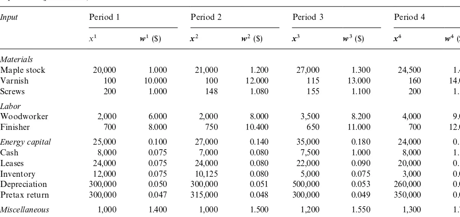
Table 2
Input data (price is in$)
Input Period 1 Period 2 Period 3 Period 4
x1 w1($) x2 w2($) x3 w3($) x4 w4($)
Materials
Maple stock 20,000 1.000 21,000 1.200 27,000 1.300 24,500 1.400
Varnish 100 10.000 100 12.000 115 13.000 160 14.000
Screws 200 1.000 148 1.080 155 1.100 200 1.130
Labor
Woodworker 2,000 6.000 2,000 8.000 3,500 8.200 4,000 9.000
Finisher 700 8.000 750 10.400 650 11.000 700 12.000
Energy capital 25,000 0.100 27,000 0.140 35,000 0.180 24,000 0.190
Cash 8,000 0.075 7,000 0.080 7,500 1.000 8,000 1.100
Leases 24,000 0.075 24,000 0.080 22,000 0.090 20,000 0.110
Inventory 12,000 0.075 10,125 0.080 5,000 0.075 3,000 0.090
Depreciation 300,000 0.050 300,000 0.051 500,000 0.053 260,000 0.060
Pretax return 300,000 0.047 315,000 0.048 300,000 0.049 350,000 0.056
Miscellaneous 1,000 1.400 1,000 1.500 1,200 1.550 1,300 1.700
Proxt $14,900 $19,400 $36,920 $26,269
Table 3
E$ciency results when the preceding period is chosen as base period
Index Period 1P2 Period 2P3 Period 3P4
IPE 1.197 1.216 1.017
OCRA 1.005 1.015 0.983
APC $2135 ($13,312) $19,656
PPP $2135 ($13,312) $19,656
Laspeyres 1.028 0.887 1.161
Paasche 1.037 0.888 1.150
Fisher 1.032 0.887 1.156
ToKrnqvist 1.032 0.889 1.158
a less rigorous setting. However, let us assume that the management of the group desires a comprehens-ive picture of the development of the production and the quality of the managerial decisions at the plant. In the calculation of the IPE index we make the additional assumption that no material is wasted, hence the value added by the unit is simply the net of revenue and cost of materials. Since the change of consumption is not proportional, this assump-tion implies that the construcassump-tion has been altered throughout the period. If not, IPE would be the only method to explicitly acknowledge this particu-lar form of input.
Indeed, it is certainly a scattered image that is presented by the eight consultants. Table 3 consists of the results from the evaluation where the
preced-ing period is chosen as base period. Notice that the
"gures for the APC and PPP Method are in dollars
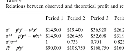
Table 4
Relations between observed and theoretical pro"t and revenue Period 1 Period 2 Period 3 Period 4 nt"ptyt!wtxt $14,900 $19,400 $36,920 $26,269 nHt"ptyH!wtxH $14,900 $26,456 $52,698 $31,932
nt/nHt 1 0.733 0.701 0.823
Rt"ptyt $90,000 $108,750 $168,750 $160,675
RHt"ptyH $90,000 $94,992 $191,250 $116,205
Rt/RHt 1 1.146 0.882 1.383
that IPE and OCRA, as opposed to the other measures, implicate productivity improvement be-tween time periods 2 and 3. It is also notable that the OCRA method, as the only method, indi-cates productivity deterioration between time peri-ods 3 and 4. The TFP based measures, i.e.
Laspeyres, Paasche, Fisher, and ToKrnqvist, are
heavily correlated and report a signi"cant decrease
in e$ciency between periods 2 and 3, around 0.89.
The APC and PPP methods record a similar dip,
here expressed as loss of$13,312. A closer look at the
data reveals out-of proportional increases of energy and maple stock consumption, which if accounted for in the IPE method would lower the score.
Halting at this point would imply that the con-clusion, ranging from deteriorating (OCRA) to
successful performance (APC), may depend
merely on the personal trust and prestige the man-agement has vested in any of the given methods (or consultants). In the general case, there exists
no correction for an e$ciency measure that
relates current performance to some arbitrary reference set. However, to create a basis for comparison, assume that we in addition to the given data in Table 1 have some knowledge about the technology of the plant and its behavior. First, introduce a minimum of notation. The production process produces an output vector y
us-ing an input vector x, facing input prices w
and output prices p. Let the output y of period 1
be the result of pro"t maximization, i.e. estimate an
inverted technology matrix T such that y1 is the
optimal solution when (pt,wt)"(p1,w1) in
prob-lem (1) below. The formulation enables the DMU to freely choose the inputs up to the observed budget level and gauge the outputs accordingly.
max nt(x,y)"pty!wtx
To update the matrixTtover the horizon, assume
that all productivity improvements originate in the corresponding activity and that there is no
com-parative di!erence between the two products. That
is, if the material consumption of maple stock in
total decreases from an expected level of 22,000 to 21,000, then this improvement updates the
techno-logy matrix symmetrically not to a!ect the product
choice problem. The optimal pro"t calculated is an
upper limit to the performance of the DMU and
assumes full#exibility in outputs and inputs. The
revenue maximization problem is de"ned in
prob-lem (2) below, where the DMU is assumed to adjust the output, given the observed input mix. If
Twould be updated in the revenue maximization
case, the observed solution would be the trivial solution to an over-determined set of equations. Thus, the technology matrix is not updated to
re-#ect the existing choice at the time before the
im-provements. This implies that a revenue higher
thanRHis attainable due to productivity changes in
the technology matrix. Subsequently, a ratio of observed to calculated revenue of 1.3 would imply 30% higher revenue than would have been
attain-able using the technology of the"rst period. Since
the inverse technology matrixT~1does not exist,
the cost minimization problem cannot be for-mulated for this example, as there is no substitution
possible in the formulation Ty5x as opposed
to T!1x
5y. The results are summarized in
Table 4 and reveal that the enterprise in the example
in fact deteriorates in terms of pro"t e$ciency, but
does a fairly good job at revenue maximization.
max Rt(y)"pty
s.t. Ty)xt,
y3R2 `.
(2)
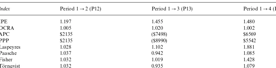
Table 5
E$ciency reported by selected di!erent methods when period 1 is chosen as base period
Index Period 1P2 (P12) Period 1P3 (P13) Period 1P4 (P14)
IPE 1.197 1.455 1.480
OCRA 1.005 1.020 1.002
APC $2135 ($7498) $6569
PPP $2135 ($8990) $5542
Laspeyres 1.028 1.102 1.881
Paasche 1.037 0.942 1.085
Fisher 1.032 1.019 1.428
ToKrnqvist 1.032 0.935 1.079
Fig. 1. The e$ciency reported by the IPE, OCRA, Fisher, Paasche and ToKrnqvist indexes (left scale) and APC, PPP in-dexes (right scale).
productivity improvement between periods 1 and 3, whereas the APC and PPP Method, and Paasche
and ToKrnqvist productivity index implicate
pro-ductivity deterioration. All methods seem to agree
that there indeed was an increase in e$ciency
be-tween the"rst and last period, although the span is
considerable from 0.2% (OCRA) to 88% (Las-peyres).
Fig. 1 depicts the graphs of the measures and the spread of recommendations is visually presented. Apparently, the results indicate that the methods are closer to revenue maximization than to true
pro"t maximization, which further supports the
"ndings in the property test. As the revenue
maxi-mization case cannot be formulated as in the
prop-erty test some caution is advised in the
interpretation of the example. However, it is
evi-dent that a managerial#aw, in this example a
sub-optimal output mix may very well be hidden be-hind piecemeal improvements of the technology
while increases in e$ciency are reported. Thus, it is
clearly of importance to know the limitations and behavior of these methods in the context of economic decision making. The rest of this
paper will propose, de"ne and apply a series of
microeconomic tests for this particular class of productivity measures, in order to highlight their limitations.
4. Economic properties for tests
Many of the properties in, e.g. Diewert [19] are primarily based on mathematical equivalence argu-ments. The shape and behavior of the index is
evaluated for its coherence with the existing body of knowledge, its mathematical tractability or as in
F+rsund [20], strong behavioral assumptions. An
example may be strict proportionality, as in
Diewert [19] and F+rsund [20], a condition that
importance in the context of long-term evaluation. Theoretical support against the use may be found even in economic theory, e.g. the saturation axiom in micro-economic utility theory.
Hence, there is a need of supplementary proper-ties that better incorporates economic relevance. In
this paper we identify a minimal set of"ve relevant
properties that a productivity index needs to satisfy to rightly assess the performance development of a DMU, viz. commensurability, monotonicity,
rev-enue maximization, cost minimization, and pro"t
maximization. The "rst two tests relate to two
fundamental properties for any performance
evalu-ation }a proportional change in all prices or no
change at all in input and output results in constant
e$ciency; and that partial improvements are
monotonically rewarded, ceteris paribus. The
omission of the"rst would lead to a built-in bias
and the second would jeopardize even the most careful use of the measure. The behavioral proper-ties related to economic performance test a
grad-ually more sophisticated economic e$ciency:
revenue e$ciency, cost e$ciency, and pro"t e$
-ciency. As they are closely related both in the math-ematical sense and from a managerial viewpoint, it
is logical to build the compound pro"t e$ciency,
where inputs and outputs are both variables, from the partial optimizations of revenue and cost. It has
been shown elsewhere (e.g. [23]) that pro"t
maxi-mization presumes the former two conditions. The following notation is introduced for the evaluation from a base periods 0 until an
evalu-ation period ¹. LetP
i(x0,xT;y0,yT;w0,wT;p0,pT)
be a generic performance measure where x0 and
xTare the input vectors for periods 0 and¹,
respec-tively,y0and yTare the output vectors for period
0 and¹,w0,wT,p0andpTare the input and output
prices associated with periods 0 and¹. The input
vector x is assumed strictly positive, whereas the
output vector y and the prices w,p are assumed
non-negative, forming positive sums wx and py.
Next, the properties are presented mathematically.
PT1 (Commensurability). The commensurability
property (PT1) re#ects the intuitively appealing
stability of a measure against systematic changes of all prices. A measure failing this test may be
sensi-tive to in#ation or the unit of measurement. The
special case when r"0, called identity elsewhere
(e.g. [19]), illustrates the case where constant action
should lead to constant ranking,ceteris paribus. If
violated for r'0, it forces the use of real rather
than nominal prices in the measure, which may
pose an additionalcaveatfor some measures.
pT"(1#r)p0'wT"(1#r)w0
NP
i(x,x;y,y;wT,w0;pT,p0)"1.
PT2 (Monotonicity). The monotonicity property
(PT2) upholds the logic of a measure. Thus, a measure not satisfying this test would make the evaluation severely hazardous. The test asserts that if inputs increase (decrease) over time, with un-changed outputs and prices, the productivity measure decreases (increases). Similarly, if outputs increase (decrease) between two time periods, the productivity measure increases (decreases):
xT"jx0NP
PT3(Revenue Maximization). The revenue e$ciency test (PT3) presumes that a DMU will choose to operate the output mix that corresponds to the highest market prices. The test states that if the revenue is increased (decreased) between time
peri-ods 0 andT, under constant input and prices, then
the productivity measure increases (decreases). That is, the condition is rather weak and merely assures that an economically sound output
adjust-ment, given "xed input, is subject to monotone
reward.
PT4(Cost Minimization). Under cost minimization
behavior the DMU will choose the input mix that best corresponds to the market prices of the inputs,
given "xed output volume and value. PT4 states
Fig. 2. Productivity change (physical units).
with invaried outputs and prices, the productivity measure increases (decreases).
wxT"j~1wx0NP
i(x0,xT;y,y;w,w;p,p)'1, wxT"jwx0NP
i(x0,xT;y,y;w,w;p,p)(1, j'1.
PT5(Pro"t Maximization). The pro"t
maximiza-tion condimaximiza-tion (PT5) states that if the pro"t is
increased (decreased) between two time periods with equal prices then the productivity measure increases (decreases). However, a common feature
of many e$ciency indexes is to enforce
propor-tionality in revenue generation, i.e. pro"ts are
as-sumed to be in relation to total inputs. The shareholders though would expect the DMU to maximize return on capital stock on long-term basis, which in case of a constant capital stock would imply maximization of absolute rather than relative pro"t.
p(yT!y0)'w(xT!x0)
NP
i(x0,xT;y0,yT;w,w;p,p)'1,
p(yT!y0)(w(xT!x0)
NP
i(x0,xT;y0,yT;w,w;p,p)(1.
Note that PT3 and PT4 are necessary but
not su$cient conditions for PT5, which
corres-ponds to the ultimate form of economic e$ciency.
Formally, we state this as a lemma to be used in the investigations.
Lemma 1 PT3 and PT4 as necessary conditions for PT5.
Proof. Follows from the de"nitions. Let (x,y0) and
(x,yT) be an observation violating P¹3. Thus it
violates the de"nition ofP¹5, sincep(yT!y0)'0
andP()))1 orp(yT!y0)(0 andP())*1.
Sim-ilarly, let (x0,y) and (xT,y) be an observation
violat-ing P¹4. This implies an analogous violation of
P¹5, since 0'w(xT!x0) andP()))1 or the
op-posite.
To get a better understanding of how the behav-ioral properties are corresponding to changes in productivity, graphical representations of the three properties are given in the next section.
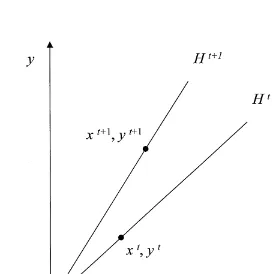
5. Graphical representation
The traditional way of seeing a productivity growth for non-frontier productivity measures is
} if we consider Fig. 2, where one input type is
required to produce one output type under
con-stant returns to scale } a change in technology
leading to a shift in the production frontier from
HttoHt`1. The productivity in the respective time
periods equals the slope of the production frontier,
and the productivity growth (e$ciency) is equal to
the ratio of the slopes. Note also that observed production in the respective time periods is equiva-lent to frontier production, since in non-frontier productivity analysis the production frontiers are estimated through observed data.
It is, however, hard to interpret the frontier shift
in production from (xt,yt) to (xt`1,yt`1) in an
eco-nomic sense } is it subject to a pro"tability
in-crease? For this purpose we scale the axes with their respective prices, thus having cost at the horizontal axis and revenue at the vertical axis (Figs. 3 and 4). This step also solves the aggregation problem, which occurs if multiple inputs and/or outputs are considered.
Observed production is still equivalent to
fron-tier production, since the fronfron-tiersGtandGt`1are
Fig. 3. Productivity change (monetary units).
Fig. 4. Productivity change (monetary units).
The mathematical description of the revenue maximization and cost minimization properties is graphically outlined in Fig. 3. It is clear from the
"gure that the considered productivity index
sup-ports revenue maximization behavior, as an in-crease in revenue with sustained cost level is subject to an increase of the slope of the production fron-tier, and vice versa. Similarly, it is also clear that the index supports a cost minimization behavior.
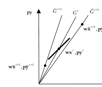
Fig. 4 visualizes the mathematical description of
the pro"t maximization test. As can be seen in the
"gure three di!erent production frontiers are
depic-ted, of which two corresponds to the last time
period (Gxt`1andGKt`1) and one to the former time
period (Gt). Included in the "gure is also an
iso-pro"t curve marked as the bold solid line. A
pro-duction point positioned upper-left of the iso-pro"t
curve is subject to an increase in DMU pro"t, and
should according to the property test be recognized as a growth in the performance measure. But if we consider the two production points in the last time
period, it is thus clear that (wxyt`1,pyyt`1) is subject
to a more e$cient production although the pro"t
has declined (below the iso-pro"t curve), whereas
(wx(t`1,py(t`1) is subject to a less e$cient
produc-tion although a greater pro"t has been achieved
(above the iso-pro"t curve).
Another interpretation is that even if the DMU chooses to produce the products that maximize
pro"t, it might not be bene"cial from an incentive
perspective. E.g., a DMU is o!ered to change
tech-nology, giving the opportunity to rise its yield but at the cost of a lower production pace. This is an
example of a situation that could lead to the
pro-duction (wxyt`1,pyyt`1in Fig. 4. We argue that it is
not the primary purpose to focus on the ratio of revenues to costs as it does not give a true picture of the situation. That is, although the index indicates a productivity increase, this increase is not
neces-sarily bene"cial for the unit.
6. Integrated Partial E7ciency,IPE
The integrated partial e$ciency (IPE) method by
Agrell and Wikner [15] is based on economically
weighted partial e$ciency measures. The method
the main characteristics of the method, pertaining to the performance index, are explained.
To best re#ect upon the resource e!ort required
to produce the respective outputs, output weights
are used. Output weight g for product n at time
periodtis de"ned as the product price subtracted
with the cost of the non-transformable inputs the product consists of, gtn"ptn!wtz8
n. Consequently,
the vector z8
n shows great similarities with a
BOM (bill of material), i.e. every component in
z8n represents the number of units that is required
of the input to produce one unit of product n.
A non-transformable input is thus an input that is not consumed by the process and hence not con-trollable by the DMU, e.g. semi-manufactures, whereas a transformable input is consumed in the process, e.g. labor. This division is crucial if the
DMU's performance is to be evaluated as it
con-trols only the amount and mix of transformable inputs used.
The total value added by the unit is calculated as<t"gtyt. The value added is then put in relation to every consumed input, i.e. partial productivity is calculated for each transformable input. The
amount of transformable inputhduring time
peri-odtis found as the net of input usage and expected
usage of the non-transformable input.
PPth"
Note that in case the input x
h is zero for all t,
then input his excluded from the evaluation.
Oc-currences of zero cause a singularity in the partial
productivity function, PP for inputhduring time
periodt.
To enable relative comparison over inputs and time, the partial productivities are normalized to
par-tial e$ciencies. Partial e$ciency is calculated as
PEth" PPth max
tMPPthN
. (5)
A measure of unity represents a fully e$cient point,
where an e$cient point implies that the unit at this
time used the input as e$ciently as possible. To
obtain a measure of the overall e$ciency with
re-spect to relevant costs, i.e. economic importance,
weighted partial e$ciency is de"ned for a unit as
(6), where the input weightcfor the transformable
inputhequals the varying cost shares of the inputs
used, see (7). Evidently, various inputs have
di!erent economic relevance. Intuitively, it is
im-portant to use the most costly inputs in the best way possible.
To capture the dynamics in the e$ciency
devel-opment over time a relative measure is used,
integrated partial e$ciency, IPE. The IPE index is
based on the Malmquist index [21] and is de"ned
as
IPEt" WPEt
WPEt~1, t*1. (8)
Proposition 1. (A) The IPE method as dexned above satisxes properties PT2, PT4 and fails in PT1, PT3 and PT5.
(B) If no division in transformables and non-formables is done, i.e. all inputs are considered trans-formables, the IPE method then satisxes PT2, PT3,
PT4 and fails in PT1 and PT5.
Not to burden the paper with details, the tech-nical proof of Proposition 1 is omitted here and so are the rest of the proofs. The technical presenta-tion underlying this paper is given in [25].
7. Operational competitiveness ratings,OCRA
The operational competitiveness ratings
(OCRA) by Parkan [14] is presented as an alterna-tive to data envelopment analysis [4]. The main thrust of OCRA is to circumvent the
implementa-tion-related di$culties with DEA. The interested
detailed description of the model and its various designs.
As opposed to most other measures OCRA
esti-mates the relativeine$ciency of a production unit,
hence ratings of above 1 implies ine$ciency
where-as ratings of unity implies e$ciency. The method is
formulated as a linear programming problem, where the goal is to minimize an unknown but
linear and increasing ine$ciency rating function
E(ct,!rt), subject to cost and revenue constraints.
If the production unit uses inputs ofKcategories,
and produce outputs of ¸categories, the problem
can be formulated as (9), where c denotes cost
(1c5wx) and r revenue (1r5py). 1 represents
a unity vector of appropriate size.
min E(ct,!rt),
Parkan [14] has shown that if the signi"cance
parameters are constant over time, i.e.atk"a
k and btl"b
l, then the ine$ciency ratings, EHt, can be
computed easily using the procedure below. He
further suggests the signi"cance parameter, a
k, to equal the varying cost shares of the inputs used to
more accurately measure the unit's ine$ciency. The
same applies tob
l, where the value of the constants
should re#ect the varying revenue shares of the
outputs produced, see (10):
a
The procedure for obtaining the performance rat-ing for a unit is as follows:
1. Compute the performance ratingCof the unit's
resource usage of categorykat time t.
Ctk"1#a
2. Compute the performance ratingRof the unit's
revenue generation of categorylat time t.
Rtl"1#b
3. Compute the overall performance rating of the
unit at time t by summing the resource and
revenue ratings, C and R, respectively, and
a subsequent scaling:
EHt" +kCtk#+lRtl min
iM+kCik#+lRilN
∀t.
Proposition 2. The OCRA method as dexned above satisxes properties PT1, PT2, PT3, PT4 and fails in PT5.
8. APC Method
The"rst of the examined measures that directly
relate a productivity change to a change in pro"
t-ability level, is the method developed by the Ameri-can Productivity Center, APC (see e.g. Belcher [12] or Miller and Rao [22]).
PT APC"
p0yT)w0x0!p0y0)w0xT
p0y0 . (11)
Proposition 3. The APC Method as dexned above satisxes properties PT1}PT4 and fails in PT5.
9. PPP Method
The PPP method (pro"tability"
productiv-ity#price recovery) by Miller [13] shows great similarities with the APC method, yet instead of using base period prices of time period 0, a method
for de#ating the present value is used (the ratio
within brackets in Eq. (12). The present value is
de#ated using a weighted approach, where the
pro-duced quantities are used as weights. It is shown by Miller and Rao [22] that if only one item is
con-sidered andthas any value, or multiple items are
Method gives identical results.
Proposition 4. The PPP Method as dexned above satisxes properties PT1}PT4 and fails in PT5.
10. Laspeyres productivity index
The Laspeyres productivity index is the oldest of the more familiar TFP indexes, and it dates back to the 19th century ([8]). It is calculated as a ratio of Laspeyres output quantity index at time period
¹to a Laspeyres input quantity index at period¹,
with time period 0 as the base period, as
PTL"QL(y0,yT,p0,pT)
L()) is the Laspeyres output quantity index,
andQ
L*()) is the Laspeyres input quantity index.
Proposition 5. The Laspeyres productivity index as dexned above satisxes properties PT1,PT2,PT3,PT4 and fails in PT5.
11. Paasche productivity index
The Paasche productivity index [9] is similar to the Laspeyres productivity index, yet the
evalu-ation period¹is used as the base period. In
accord-ance with the Laspeyres TFP index the Paasche
TFP index is de"ned as the ratio of the output
quantity index to the input quantity index, see (14),
whereQ
P()) is the Paasche output quantity index,
andQH
P()) is the Paasche input quantity index:
PTP"QP(y0,yT,p0,pT)
Proposition 6. The Paasche productivity index as dexned above satisxes properties PT1}PT4 and fails in PT5.
12. Fisher productivity index
The Fischer productivity index [26] is de"ned as
the ratio of the Fisher output quantity index to the Fisher input quantity index, as
PTF"QF(y0,yT,p0,pT)
ty index and input quantity index, respectively. By (15) it is shown that the Fisher productivity index is the geometric mean of the Laspeyres and Paasche TFP indexes.
Proposition 7. The Fisher productivity index as
de-xned above satisxes properties PT1}PT4 and fails in PT5.
13. ToKrnqvist productivity index
The ToKrnqvist productivity index [11] is
cal-culated similarly to the three preceding TFP in-dexes, as the ratio of the output quantity index to the input quantity index.
PTT"QT(y0,yT,p0,pT)
index and input quantity index, respectively.A
nfor
time periodtis the periodtrevenue share of output
n, andB
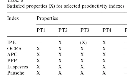
Table 6
Satis"ed properties (X) for selected productivity indexes Index Properties
PT1 PT2 PT3 PT4 PT5
IPE * X (X) X *
Proposition 8. The To(rnqvist productivity index as dexned above satisxes properties PT1,PT2 and fails in PT3}PT5.
14. Conclusion
Converting the multi-dimensional nature of productivity into a scalar number requires a careful construction of the aggregation measure. The temptation to apply an index-number-based pro-ductivity measure to evaluate managerial perfor-mance may come at a price in terms of ambiguous interpretation and non-economical conclusions. As always, the low requirements on information by the methods correspond largely to a lack of detail in the information output. In fact, the knowledge re-quired to correctly interpret the productivity in-dexes is higher than for the more elaborate parametric or frontier-based models. In order to highlight the shortcomings of the productivity in-dexes in their application to managerial decision making, we choose to benchmark the benchmarks. Five properties of relevance for a business or industry in open competition have been suggested, among those behavioral properties such as
maximi-zation of revenue and pro"t and minimization of
cost, and also stability properties such as sensitivity to proportional price changes and monotonicity. All of the properties are such that a DMU could be assumed to behave in accordance with them under
reasonable assumptions such as pro"t
maximiza-tion. Eight common productivity indexes: four Total Factor Productivity (TFP) indexes
Las-peyres, Paasche, Fisher, and ToKrnqvist; the
Ameri-can Productivity Center-method (APC); the
`Pro"tability"Productivity#Price recoverya
-method (PPP); Operational Competitiveness
Rat-ings (OCRA); and Integrated Partial E$ciency
(IPE), are tested and the results are given in Table 6. Apparently, all selected indexes satisfy the funda-mental property PT2 (monotonicity). All measures, save IPE, satisfy PT1 (commensurability) and also
the partial optimization measures PT3 and PT4 are
covered by most measures except the ToKrnqvist
index. However, the perhaps most important test,
PT5, pro"t maximization, is not covered by any
presented index. This is particularly noteworthy as
the pro"t maximization assumption is used by Balk
[16] and FaKre and Grosskopf [23] to compare the
Malmquist and ToKrnqvist indexes. The result
pro-vides an interesting incentive basis, in particular when the measure is applied in addition to purely
"nancial rewards, such as pro"t sharing, stock
op-tions, convertible stock and provision funds. As the productivity in this matter may pose as an
alterna-tive to short-term pro"tability, an interesting issue
is how important the respective incentive compo-nents should be to promote long-term organiza-tional goals. A possible objection against the
approach may be that productivity and pro"
tabil-ity are two substantially di!erent concepts and no
measure could be devised that satisfactorily covers them both. If so, then the relevance of the index-number and TFP approach must also be ques-tioned, as the use of exogenous prices indeed attempts to evaluate something in addition to
merely technical e$ciency. There seems to be a
fu-tile exercise to convince the business that the be-havior of a particular measure would be a better measure of future economic performance than the demonstrated ability to gauge inputs and outputs
as to maximize pro"ts during some reasonable
horizon. As illustrated in the example, the con-clusions drawn from the measures may in many cases contradict economic common sense. In
attempt to explore operationalewectiveness, rather
than merelyezciency.
Acknowledgements
The research reported in this paper was partly supported by grants from Sciences the Swedish Foundation for Strategic Research.
References
[1] P. Bogetoft, Incentive e$cient production frontiers: an agency perspective on DEA, Management Science 40 (8) (1994) 959}968.
[2] P. Bogetoft, Incentives and productivity measurements, In-ternational Journal of Production Economics 39 (1995) 67}81.
[3] W.E. Diewert. Index number issue in incentive regulation. Discussion paper 93-06, Department of Economics, University of British Columbia, Vancouver, 1993. [4] A. Charnes, W.W. Cooper, E. Rhodes, Measuring the
e$ciency of decision making units, European Journal of Operational Research 2 (6) (1978) 429}444.
[5] D. Caves, L. Christensen, W.E. Diewert, The economic theory of index numbers and the measurement of input, output and productivity, Journal of Economic Theory 64 (2) (1982) 554}567.
[6] N. Balk, Malmquist productivity indexes and Fisher ideal indexes: Comment, Economic Journal 103 (1993) 680}682. [7] R. FaKre, S. Grosskopf, Malmquist indexes and Fisher ideal
indexes, Economic Journal 102 (1992) 158}160.
[8] E. Laspeyres, Die Berechnung einer mittleren Warenpreis-steigerung. JahrbuKcher fuKr NationaloKkonomie und Statis-tik, 16 (1871) 296}314 (In German).
[9] H. Paasche. UGber die Preisentwicklung der letzen Jahre nach den Hamburger BoKrsennotierungen. JahrbuKcher fuKr National-oKkonomie and Statistik 23 (1874) 168}178. (In German) [10] I. Fisher, The Making of Index Numbers: A Study of
Their Varieties, Tests, and Reliability, Houghton Mi%in, Boston, 1922.
[11] L. ToKrnqvist, The bank of Finland's consumption price index, Bank of Finland Monthly Bulletin 10 (1936) 1}8.
[12] J.G. Belcher Jr, The Productivity Management Process, American Productivity Center, Houston, 1984.
[13] D.M. Miller, Pro"tability"productivity#price recov-ery. Harvard Business Review 62 (3) (1984) 145}153. [14] C. Parkan, Operational competitiveness ratings of
produc-tion units, Managerial and Decision Economics 15 (3) (1994) 201}221.
[15] P.J. Agrell, J. Wikner, A coherent methodology for productivity analysis employing integrated partial e$ cien-cy, International Journal of Production Economics 46}47 (1996) 401}411.
[16] R.S. FaKre, C.A.K. Grosskopf, Lowell, Production Fron-tiers, Cambridge University Press, Cambridge, 1994. [17] R. Frisch, Annual survey of general economic theory:
The problem of index numbers, Econometrica 4 (1936) 1}38.
[18] W. Eichhorn, J. Voeller, Theory of the price index, Spring-er, Berlin, 1976.
[19] W.E. Diewert, Fisher ideal output, input, and productivity indexes revisited, Journal of Productivity Analysis 3 (3) (1992) 211}248.
[20] F.R. F+rsund. The Malmquist productivity index, TFP and scale. Memorandum no. 233, Department of Econ-omics, GoKteborg University, 1997.
[21] S. Malmquist, Index numbers and indi!erence surfaces, Trabajos de Estatistica 4 (1953) 209}242.
[22] D.M. Miller, P.M. Rao, Analysis of pro"t-linked total-factor productivity measurement models at the"rm level, Management Science 35 (6) (1989) 757}767.
[23] R. FaKre, S. Grosskopf, Intertemporal Production Fron-tiers: With Dynamic DEA, Kluwer, Boston, 1996. [24] J. Wikner, P.J. Agrell. Evaluation of systems with
bottle-necks employing integrated partial e$ciency. Working Paper WP-242, Department of Production Economics, LinkoKping Institute of Technology, 1997.
[25] P.J. Agrell, B.M. West. On microeconomic rationality and non-frontier e$ciency, Working Paper WP-251, Depart-ment of Production Economics, LinkoKping Institute of Technology, 1998.