The Essential R Reference Ebook free dowwnload

The

ESSENTIAL

R

The

ESSENTIAL

R

REFERENCE

The Essential R Reference

Published by

John Wiley & Sons, Inc. 10475 Crosspoint Boulevard Indianapolis, IN 46256

www.wiley.com

Copyright © 2013 by Mark Gardener

Published by John Wiley & Sons, Inc., Indianapolis, Indiana Published simultaneously in Canada

ISBN: 978-1-118-39141-9 ISBN: 978-1-118-39140-2 (ebk) ISBN: 978-1-118-39138-9 (ebk) ISBN: 978-1-118-39139-6 (ebk)

Manufactured in the United States of America

10 9 8 7 6 5 4 3 2 1

No part of this publication may be reproduced, stored in a retrieval system or transmitted in any form or by any means, electronic, mechanical, photocopying, recording, scanning or otherwise, except as permitted under Sections 107 or 108 of the 1976 United States Copyright Act, without either the prior written permission of the Publisher, or authorization through payment of the appropriate per-copy fee to the Copyright Clearance Center, 222 Rosewood Drive, Danvers, MA 01923, (978) 750-8400, fax (978) 646-8600. Requests to the Publisher for permission should be addressed to the Permissions Department, John Wiley & Sons, Inc., 111 River Street, Hoboken, NJ 07030, (201) 748-6011, fax (201) 748-6008, or online at http://www.wiley.com/go/permissions.

Limit of Liability/Disclaimer of Warranty: The publisher and the author make no representations or warranties with respect to the

accuracy or completeness of the contents of this work and specifically disclaim all warranties, including without limitation warranties of fitness for a particular purpose. No warranty may be created or extended by sales or promotional materials. The advice and strategies contained herein may not be suitable for every situation. This work is sold with the understanding that the publisher is not engaged in rendering legal, accounting, or other professional services. If professional assistance is required, the services of a competent professional person should be sought. Neither the publisher nor the author shall be liable for damages arising herefrom. The fact that an organization or Web site is referred to in this work as a citation and/or a potential source of further information does not mean that the author or the publisher endorses the information the organization or website may provide or recommendations it may make. Further, readers should be aware that Internet websites listed in this work may have changed or disappeared between when this work was written and when it is read.

For general information on our other products and services please contact our Customer Care Department within the United States at (877) 762-2974, outside the United States at (317) 572-3993 or fax (317) 572-4002.

Wiley publishes in a variety of print and electronic formats and by print-on-demand. Some material included with standard print versions of this book may not be included in e-books or in print-on-demand. If this book refers to media such as a CD or DVD that is not included in the version you purchased, you may download this material at http://booksupport.wiley.com. For more information about Wiley products, visit www.wiley.com.

Library of Congress Control Number: 2012948918

Trademarks: Wiley and the Wiley logo are trademarks or registered trademarks of John Wiley & Sons, Inc. and/or its affiliates, in the

There's only one corner of the universe

you can be certain of improving, and

that's your own self.

ABOUT THE AUTHOR

Mark Gardener

(

http://www.gardenersown.co.uk

) is an

ecologist, lecturer, and writer working in the UK. He has a passion for

the natural world and for learning new things. Originally he worked

in optics, but returned to education in 1996 and eventually gained his

doctorate in ecology and evolutionary biology. This work involved a

lot of data analysis and he became interested in R as a tool to help in

research. He is currently self-employed and runs courses in ecology,

data analysis, and R for a variety of organizations. Mark lives in rural

Devon with his wife Christine (a biochemist) and still enjoys the

natu-ral world and learning new things.

ABOUT THE TECHNICAL EDITOR

Executive Editor

Carol Long

Project Editor

Victoria Swider

Technical Editor

Richard Rowe

Production Editor

Kathleen Wisor

Copy Editor

Kim Cofer

Editorial Manager

Mary Beth Wakefield

Freelancer Editorial Manager

Rosemarie Graham

Associate Director of Marketing

David Mayhew

Marketing Manager

Ashley Zurcher

Business Manager

Amy Knies

Production Manager

Tim Tate

Vice President and Executive Group

Publisher

Richard Swadley

Vice President and Executive Publisher

Neil Edde

Associate Publisher

Jim Minatel

Project Coordinator, Cover

Katie Crocker

Compositor

Jeff Lytle, Happenstance Type-O-Rama

Proofreader

James Saturnio, Word One

Indexer

Jack Lewis

Cover Designer

Ryan Sneed

ACKNOWLEDGMENTS

First of all my thanks go out to the R project team and the many authors and programmers who

work tirelessly to make this a peerless program. I would also like to thank my wife, Christine,

who has had to put up with me during this entire process, and in many senses became an

R-widow! Thanks to Wiley, for helping this book become a reality, especially Carol Long and

Victoria Swider. I couldn’t have done it without you. Thanks also to Richard Rowe, the technical

reviewer, who first brought my attention to R and its compelling (and rather addictive) power.

Last but not least, thanks to the R community in general. I learned to use R largely by trial and

error and using the vast wealth of knowledge that is in this community. I hope that this book is a

worthwhile addition to the R knowledge base and that it will prove useful to all users of R.

INTRODUCTION

R

is rapidly becoming the

de facto

standard among professionals, and is

used in every conceivable discipline from science and medicine to

busi-ness and engineering. R is more than just a computer program; it is a

statisti-cal programming environment and language. R is free and open source and is,

therefore, available to everyone with a computer.

R is a language with its own vocabulary and grammar. To make R work for you, you

com-municate with the computer using the language of R and tell it what to do. You accomplish this

by typing commands directly into the program. This means that you need to know some of the

words of the language and how to put them together to make a “sentence” that R understands.

This book aims to help with this task by providing a “dictionary” of words that R understands.

The help system built into R is extensive, but it is arranged by command name; this makes it

hard to use unless you know some command names to start with. That’s where this book comes

in handy; the command names (the vocabulary of R) are arranged by topic, so you can look up

the kind of task that you require and find the correct R command for your needs.

I like to think of this book as a cross between a dictionary, a thesaurus, and a glossary, with a

fair sprinkling of practical examples. Even though some may consider me an “R expert” at this

point, I am still learning and still forgetting! I often have to refer to notes to remind me how

to carry out a task in R. That is why I wrote this book—to help novice users learn more easily,

and to provide more experienced users with a reference work they can delve into time and time

again. I also learned a great deal more about R by writing about it, and I hope that you will find it

an essential companion in your day-to-day conversations with R.

Who This Book Is For

This book is for anyone who needs to analyze any data, whatever their discipline or line of work.

Whether you are in science, business, medicine, or engineering, you will have data to analyze

and results to present. R is powerful and flexible and completely cross-platform. This means you

can share data and results with anyone. R is backed by a huge project team, so being free does not

mean being inferior!

Beginning R: The Statistical Programming Language

, which provides a different learning

environ-ment by taking you from simple tasks to more complex ones in a linear fashion.

If you are already familiar with R, this book will help as a useful reference work that you can

call upon time and time again. It is easy to forget the name of a command or the exact syntax of

the command. In addition to jogging your memory, the examples in the book will help put the

commands into context.

What This Book Covers

Each command listed in this book has an explanation of what the command does and how to use

it—the “grammar,” if you will. Related commands are also listed, as in a thesaurus, so if the word

you are looking at is not quite what you need, you are likely to see the correct one nearby.

I can’t pretend that this reference book covers every command in the R language, but it covers

a lot (more than 400). I’ve also not covered some of the more obscure parameters (formally called

“arguments” in R) for some of the commands. I called this book “Essential” because I believe it

covers the essentials. I also hope that you will find it essential in your day-to-day use of R.

One of the weaknesses of the R help system is that some of the examples are hard to follow, so

each command listed in this book is accompanied by various examples. These show you the

com-mand “in action” and hopefully help you to gain a better understanding of how the comcom-mand

works. The examples are written in R code and set out as if you had typed them into R yourself.

And unlike the built-in help system in R, you get to see the results, too!

How This Book Is Structured

This book is not a conventional textbook; it is intended as a reference work that you can delve

into at any point.

This book is organized in a topic-led, logical manner so that you can look for the kind of task that

you want to carry out in R and find the command you need to carry out that task as easily as

pos-sible, even if you do not know the name of the command. The book is split into four grand themes:

■

Theme 1: “Data”

■

Theme 2: “Math and Statistics”

■

Theme 3: “Graphics”

■

Theme 4: “Utilities”

These are hopefully self-explanatory, with the exception perhaps of “Utilities”; this covers the

commands that did not fit easily into one of the other themes, particularly those relating to the

programming side of R.

You can use the table of contents to find your way to the topic that matches the task you want

to undertake. If the command you need is not where you first look, there is a good chance that

the command you did find will have a link to the appropriate topic or command (some

com-mands have entries on more than one topic).

The following is a brief description of each of the four main themes:

Theme 1: “Data”

—This theme is concerned with aspects of dealing with data. In particular:

■

Data types

—Different kinds of data and converting one kind of data into another kind.

■

Creating data

—Commands for making data items from the keyboard.

■

Importing data

—Getting data from sources on disk.

■

Saving data

—How to save your work.

■

Viewing data

—Seeing what data you have in R.

■

Summarizing data

—Ways of summarizing data objects. Some of these commands

also appear in Theme 2, “Math and Statistics.”

■

Distribution of data

—Looking at different data distributions and the commands

associated with them, including random numbers.

Theme 2: “Math and Statistics”

—This theme covers the commands that deal with math and

statistical routines:

■

Mathematical operations

—Various kinds of math, including complex numbers,

matrix math, and trigonometry.

■

Summary statistics

—Summarizing data; some of these commands are also in Theme 1,

“Data.”

■

Differences tests

—Statistical tests for differences in samples.

■

Correlations and associations

—Including covariance and goodness of fit tests.

■

Analysis of variance and linear modeling

—Many of the commands associated with

ANOVA and linear modeling can be pressed into service for other analyses.

■

Miscellaneous Tests

—Non-linear modeling, cluster analysis, time series, and ordination.

Theme 3: “Graphics”

—This theme covers the graphical aspects of the R language:

■

Making graphs

—How to create a wide variety of basic graphs.

■

Adding to graphs

—How to add various components to graphs, such as titles,

addi-tional points, and shapes.

■

Graphical parameters

—How to embellish and alter the appearance of graphs,

includ-ing how to create multiple graphs in one window.

Theme 4: “Utilities”

—This theme covers topics that do not fit easily into the other themes:

■

Installing R

—Notes on installing R and additional packages of R commands.

■

Using R

—Accessing the help system, history of previously typed commands,

manag-ing packages, and more.

■

Programming

—Commands that are used mostly in the production of custom

Each of the topics is also split into subtopics to help you navigate your way to the command(s)

you need. Each command has an entry that is split into the following sections:

■

Command Name

—Name of the command and a brief description of what it does.

■

Common Usage

—Illustrates how the command looks with commonly used options. Use

this section as a memory-jogger; if you need fine details you can look in the “Command

Parameters” section.

■

Related Commands

—A list of related commands along with the page numbers or a link to

their entries so you can easily cross-reference.

■

Command Parameters

—Details of commonly used parameters for the command along

with an explanation of what they do.

■

Examples

—Examples of the command in action. The section is set out in code style as if

you had typed the commands from the keyboard yourself. You also see the resulting output

that R produces (including graphical output).

Some commands are relevant to more than one theme or section; those commands either have

a cross-reference and/or have an entry in each applicable place.

What You Need to Use This Book

R is cross-platform technology and so whatever computer you use, you should be able to run the

program. R is a huge, open-source project and is changing all the time. However, the basic

com-mands have altered little, and you should find this book relevant for whatever version you are

using. I wrote this book using Mac R version 2.12.1, Windows R version 2.14.2, and Linux R

version 2.14.1.

Having said that, if your version of R is older than about 2009, I recommend getting a

newer version.

Conventions

To help you get the most from the text and keep track of what’s happening, we’ve used a number

of conventions throughout the book.

R CODE

The commands you need to type into R and the output you get from R are shown in a

monospace

font. Each example that shows lines that are typed by the user begins with the

>

symbol, which

mimics the R cursor like so:

> help()

Lines that begin with something other than the

>

symbol represent the output from R (but

look out for typed lines that are long and spread over more than one line). In the following

exam-ple the first line was typed by the user and the second line is the result:

ANNOTATIONS

The hash symbol (

#

) is used as an annotation character in R (see the following example).

Anything that follows is ignored by R until it encounters a new line character. The examples used

throughout this book contain plenty of annotations to help guide you through the complexities

and facilitate your understanding of the code lines.

## Some lines begin with hash symbols; that entire line is ignored by R. ## This allows you to see the commands in action with blow by blow notes. > help(help) # This line has an annotation after the command

OPERATIONAL ASSIGNMENT

R uses two forms of “assignment.” The original form (the form preferred by many programmers)

uses a kind of arrow like so:

<-

. This is used to indicate an assignment that runs from right to left.

For example:

> x <- 23

This assigns the value

23

to a variable named

x

. An alternative form of assignment is

math-ematical type of assignment, the equals sign (

=

):

> x = 23

In most cases the two are equivalent and which you use is entirely up to you. Most of the help

examples found in R and on the Internet use the arrow (

<-

). Throughout this book I have tended

to use the

=

operator (because that is what I am used to), unless

<-

is the only way to make the

command work.

COMMAND PARAMETERS

Most R commands accept various parameters; you can think of them as additional instructions

that make the command work in various ways. Some parameters have default values that are

used if you do not explicitly indicate an alternative. These parameters are also “order specific.”

This means that you can specify the value you want the parameter to take without naming it as

long as the values are in the correct order. An example should clarify this; the

rnorm

command

generates random numbers from the normal distribution. The full command looks like this:

rnorm(n, mean = 0, sd = 1)

You supply

n

, the number of random values you want;

mean

, the mean of the values; and

sd

, the

standard deviation. Both the

mean

and

sd

parameters have defaults, which are used if you do not

specify them explicitly. You can run this command by typing any of the following:

> rnorm(n = 10, mean = 0, sd = 1) > rnorm(10, 0, 1)

> rnorm(10)

This is useful for programming and using R because it means you can avoid a lot of typing.

However, if you are trying to learn R it can be confusing because you might not remember what

all the parameters are.

Some commands will also accept the name of the parameters in abbreviated form; others will

not. In this book I have tried to use the full version of commands in the examples; I hope that

this will help clarify matters.

CROSS-REFERENCES

You can find many cross-references in this book in addition to the commands listed in the

“Related Commands” section of each command’s entry. These cross-references look like this:

the magnifying glass icon indicates a cross reference.

Cross references are used in the following instances:

■

Relevant commands in the same section or a different section.

■

Relevant sections in the same theme or in a different theme.

■

An instance in which the command in question appears in another theme or section.

■

An instance in which the command in question has related information in another theme.

Data Downloads

If you come across a command that has an example you would like to try on your own, you can

follow along by manually typing the example into your own version of R. Some of these examples

use sample data that is available for download at

http://www.wiley.com/go/EssentialRReference

.

You will find all examples that require the data are accompanied by a download icon and note

indicating the name of the file so you know it’s available for download and can easily locate it in

the download file. The download notes look like this:

the download icon indicates an example that uses data you need to download.

Once at the site, simply locate the book’s title and click the Download Code link on the book’s

detail page to obtain all the example data for the book.

There will only be one file to download and it is called

Essential.RData

. This one file contains

the example data sets you need for the whole book; it contains very few because I have tried to

make all data fairly simple and short so that you can type it directly. Once you have the file on

your computer you can load it into R by one of several methods:

■

For Windows or Mac you can drag the

Essential.RData

file icon onto the R program icon;

■

If you have Windows or Macintosh you can also load the file using menu commands or use

a command typed into R:

■

For Windows use File 

a

 Load Workspace, or type the following command in R:

> load(file.choose())

■

For Mac use Workspace 

a

 Load Workspace File, or type the following command in R

(same as in Windows):

> load(file.choose())

■

If you have Linux, you can use the

load()

command but you must specify the filename (in

quotes) exactly. For example:

> load(“Essential.RData”)

The

Essential.RData

file must be in your default working directory and if it is not, you must

THEME 1: DATA

R

is an

object-oriented language

; that means that it deals with named

objects. Most often these objects are the data that you are analyzing. This

theme deals with making, getting, saving, examining, and manipulating data

objects.

Topics in this Theme

❯

Data types (p. 3)

❯

Creating Data (p. 22)

❯

Importing Data (p. 39)

❯

saving Data (p. 49)

❯

Viewing Data (p. 61)

❯

summarizing Data (p. 121)

❯

Distribution of Data (p. 146)

COMMANDS IN THIS THEME:

case.names

(p. 78)

cbind

(p. 33)

character

(p. 5)

class

(p. 79)

colMeans

(p. 124)

colnames

(p. 80)

colSums

(p. 124)

comment

(p. 81)

cummax

(p. 172)

cummin

(p. 172)

cumprod

(p. 172)

cumsum

(p. 172)

data

(p. 46)

data.frame

(p. 6, 34)

detach

(p. 63)

dget

(p. 39)

dim

(p. 83)

dimnames

(p. 84)

dir

(p. 64)

dput

(p. 52)

droplevels

(p. 111)

dump

(p. 53)

dxxxx

(p. 148)

ecdf

(p. 152)

factor

(p. 7)

file.choose

(p. 40)

fivenum

(p. 224)

ftable

(p. 138)

getwd

(p. 65)

gl

(p. 23)

head

(p. 65)

inherits

(p. 18)

integer

(p. 8)

interaction

(p. 24)

IQR

(p. 225)

is

(p. 19)

is.xxxx

(p. 20)

lapply

(p. 126)

length

(p. 127)

levels

(p. 86)

list

(p. 9)

list.files

(p. 64)

load

(p. 47)

logical

(p. 9)

ls

(p. 67)

ls.str

(p. 87)

lsf.str

(p. 89)

mad

(p. 226)

margin.table

(p. 140)

matrix

(p. 10)

mean

(p. 227)

median

(p. 228)

mode

(p. 89)

names

(p. 90)

NCOL

(p. 92)

ncol

(p. 92)

nlevels

(p. 93)

NROW

(p. 92)

nrow

(p. 92)

numeric

(p. 11)

objects

(p. 67)

order

(p. 117)

prop.table

(p. 141)

ptukey

(p. 154)

pxxxx

(p. 155)

qtukey

(p. 158)

quantile

(p. 229)

qxxxx

(p. 159)

range

(p. 230)

rank

(p. 119)

raw

(p. 12)

rbind

(p. 36)

read.csv

(p. 40)

read.csv2

(p. 40)

read.delim

(p. 40)

read.delim2

(p. 40)

read.spss

(p. 48)

read.table

(p. 40)

read.xls

(p. 48)

read.xlsx

(p. 49)

relevel

(p. 95)

remove

(p. 68)

reorder

(p. 96)

resample

(p. 112)

rep

(p. 26)

rm

(p. 68)

RNGkind

(p. 161)

row.names

(p. 99)

rowMeans

(p. 124)

rownames

(p. 100)

rowsum

(p. 130)

rowSums

(p. 124)

rxxxx

(p. 162)

sample

(p. 113)

sapply

(p. 131)

save

(p. 59)

save.image

(p. 59)

scan

(p. 43)

sd

(p. 132, 231)

search

(p. 69)

seq

(p. 27)

seq_along

(p. 27)

seq_len

(p. 27)

set.seed

(p. 165)

setwd

(p. 70)

sort

(p. 120)

source

(p. 45)

storage.mode

(p. 101)

str

(p. 102)

subset

(p. 114)

sum

(p. 232)

summary

(p. 132)

sweep

(p. 134)

table

(p. 12)

tabulate

(p. 144)

tail

(p. 71)

tapply

(p. 135)

ts

(p. 13)

typeof

(p. 103)

unclass

(p. 104)

unlist

(p. 105)

var

(p. 235)

variable.names

(p. 106)

vector

(p. 15)

THEME

1

: D

A

T

A

Data Types

R recognizes many kinds of data, and these data can be in one of several forms. This topic shows

you the commands relating to the kinds of data and how to switch objects from one form to

another.

WHAT’S IN THIS TOPIC:

■

Types of data

(p. 3)

■

The different types/forms of data objects

■

Creating blank data objects

■

Altering data types

(p. 16)

■

Switching data from one type to another

■

Testing data types

(p. 18)

■

How to tell what type an object is

TYPES OF DATA

Data can exist as different types and forms. These have different properties and can be coerced

from one type/form into another.

COMMAND NAME

array

An

array

is a multidimensional object.

SEE

drop

for reducing dimensions of arrays in theme 2, “Math and statistics: Matrix

Math.”

Common Usage

array(data = NA, dim = length(data), dimnames = NULL)

Related Commands

Command Parameters

data = NA

A vector to be used to create the array. Other objects are coerced to

form a vector before making the array.

dim = length(data)

The dimensions of the array as a vector. A vector of 2 sets row and

column sizes, respectively.

dimnames = NULL

A list of names for each dimension of the array. The default,

NULL

, creates

no names.

Examples

## Simple arrays

> array(1:12) # Simple 12-item vector [1] 1 2 3 4 5 6 7 8 9 10 11 12

> array(1:12, dim = 12) # Set length explicitly [1] 1 2 3 4 5 6 7 8 9 10 11 12

> array(1:12, dim = 6) # Can set length to shorter than data [1] 1 2 3 4 5 6

> array(1:12, dim = 18) # Longer arrays recycle values to fill [1] 1 2 3 4 5 6 7 8 9 10 11 12 1 2 3 4 5 6

> array(1:24, dim = c(3, 4, 2)) # A 3-dimensional array , , 1

[,1] [,2] [,3] [,4] [1,] 1 4 7 10 [2,] 2 5 8 11 [3,] 3 6 9 12

, , 2

[,1] [,2] [,3] [,4] [1,] 13 16 19 22 [2,] 14 17 20 23 [3,] 15 18 21 24

## Arrays with names ## A vector

> array(1:12, dim = 12, dimnames = list(LETTERS[1:12])) A B C D E F G H I J K L

1 2 3 4 5 6 7 8 9 10 11 12

## A matrix

THEME

> array(1:24, dim = c(3, 4, 2), dimnames = list(letters[1:3], LETTERS[1:4], month.abb[1:2]))

Data in text form (not numbers) is called

character

data. The command creates a blank data

object containing empty text data items.

Common Usage

Examples

## Make a 5-item vector containing blank entries > (newchar = character(length = 5))

[1] "" "" "" "" ""

COMMAND NAME

data.frame

SEE

also

data.frame

in “Adding to existing Data.”

A

data.frame

is a two-dimensional, rectangular object that contains columns and rows. The

col-umns can contain data of different types (some colcol-umns can be numbers and others text). The

command makes a data frame from named objects.

Common Usage

data.frame(..., row.names = NULL,

stringsAsFactors = default.stringsAsFactors())

Related Commands

matrix

(p. 10)

list

(p. 9)

table

(p. 12)

Command Parameters

...

Items to be used in the construction of the data frame. Can be object

names separated by commas.

row.names = NULL

Specifies which column will act as row names for the final data frame.

Can be an integer or character string.

stringsAsFactors

A logical value,

TRUE

or

FALSE

. Should character values be converted to

factor

? Default is

TRUE

.

Examples

## Make some data

> abundance = c(12, 15, 17, 11, 15, 8, 9, 7, 9) > cutting = c(rep("mow", 5), rep("unmow", 4))

THEME

1

: D

A

T

A

## Make data frame with cutting as character data

> graze2 = data.frame(abundance, cutting, stringsAsFactors = FALSE)

## Make row names

> quadrat = c("Q1", "Q2", "Q3", "Q4", "Q5", "Q6", "Q7", "Q8", "Q9")

## Either command sets quadrat to be row names

> graze3 = data.frame(abundance, cutting, quadrat, row.names = 3) > graze3 = data.frame(abundance, cutting, quadrat, row.names = "quadrat")

COMMAND NAME

factor

This command creates

factor

objects. These appear without quotation marks and are used in

data analyses to indicate levels of a treatment variable.

SEE

subset

for selecting sub-sets and

droplevels

for omitting unused levels.

Common Usage

factor(x = character(), levels, labels = levels)

Related Commands

as.factor

(p. 16)

is.factor

(p. 20)

character

(p. 5)

numeric

(p. 11)

gl

(p. 23)

rep

(p. 26)

interaction

(p. 24)

Command Parameters

x = character()

A vector of data, usually simple integer values.

levels

Optional. A vector of values that the different levels of the factor could be.

The default is to number them in alphabetical order.

labels = levels

Optional. A vector of labels for the different levels of the factor.

Examples

## Make an unnamed factor with 2 levels > factor(c(rep(1, 5), rep(2, 4))) [1] 1 1 1 1 1 2 2 2 2

## Give the levels names

> factor(c(rep(1, 5), rep(2, 4)), labels = c("mow", "unmow")) [1] mow mow mow mow mow unmow unmow unmow unmow Levels: mow unmow

## Same as previous

> factor(c(rep("mow", 5), c(rep("unmow", 4))))

## Change the order of the names of the levels

> factor(c(rep(1, 5), rep(2, 4)), labels = c("mow", "unmow"), levels = c(2,1)) [1] unmow unmow unmow unmow unmow mow mow mow mow

Levels: mow unmow

COMMAND NAME

ftable

Creates a “flat” contingency table.

SEE

ftable

in “summary tables.”

COMMAND NAME

integer

Data objects that are numeric (not text) and contain no decimals are called

integer

objects. The

command creates a vector containing the specified number of 0s.

Common Usage

integer(length = 0)

Related Commands

as.integer

(p. 16)

is.integer

(p. 20)

character

(p. 5)

factor

(p. 7)

Command Parameters

length = 0

Sets the number of items to be created in the new vector. The default is 0.

Examples

THEME

1

: D

A

T

A

COMMAND NAME

list

A

list

object is a collection of other R objects simply bundled together. A list can be composed

of objects of differing types and lengths. The command makes a list from named objects.

Common Usage

list(...)

Related Commands

vector

(p. 15)

as.list

(p. 16)

is.list

(p. 20)

unlist

(p. 105)

data.frame

(p. 6, 34)

matrix

(p. 10)

Command Parameters

...

Objects to be bundled together as a list. Usually named objects are separated by commas.

Examples

## Create 3 vectors > mow = c(12, 15, 17, 11, 15) > unmow = c(8, 9, 7, 9) > chars = LETTERS[1:5]

## Make list from vectors

> mylist = list(mow, unmow, chars) # elements are unnamed

## Make list and assign names

> mylist = list(mow = mow, unmow = unmow, chars = chars)

COMMAND NAME

logical

A

logical

value is either

TRUE

or

FALSE

. The command creates a vector of logical values (all set

to

FALSE

).

Common Usage

logical(length = 0)

Related Commands

Command Parameters

length = 0

The length of the new vector. Defaults to 0.

Examples

## Make a 4-item vector containing logical results > logical(length = 4)

[1] FALSE FALSE FALSE FALSE

COMMAND NAME

matrix

A

matrix

is a two-dimensional, rectangular object with rows and columns. A

matrix

can contain

data of only one type (either all text or all numbers). The command creates a

matrix

object from data.

SEE

also

matrix

in “Adding to existing Data.”

Common Usage

matrix(data = NA, nrow = 1, ncol = 1, byrow = FALSE, dimnames = NULL)

Related Commands

data.frame

(p. 6, 34)

as.matrix

(p. 16)

is.matrix

(p. 20)

cbind

(p. 33)

rbind

(p. 36)

nrow

(p. 92)

ncol

(p. 92)

dimnames

(p. 84)

colnames

(p. 80)

rownames

(p. 100)

dim

(p. 83)

Command Parameters

data = NA

The data to be used to make the matrix. Usually a vector of values

(numbers or text).

nrow = 1

The number of rows into which to split the data. Defaults to 1.

ncol = 1

The number of columns into which to split the data. Defaults to 1.

byrow = FALSE

The new matrix is created from the data column-by-column by default. Use

byrow = TRUE

to fill up the matrix row-by-row.

dimnames = NULL

Sets names for the rows and columns. The default is

NULL

. To set names, use

THEME

> values = 1:12 # A simple numeric vector (numbers 1 to 12)

## A matrix with 3 columns > matrix(values, ncol = 3) [,1] [,2] [,3] > matrix(values, ncol = 3, byrow = TRUE) [,1] [,2] [,3]

> rnam = LETTERS[1:4] # Uppercase letters A-D > cnam = letters[1:3] # Lowercase letters a-c

## Set row and column names in new matrix

> matrix(values, ncol = 3, dimnames = list(rnam, cnam)) a b c

Data that are

numeric

are numbers that may contain decimals (not

integer

values). The command

creates a new vector of numbers (all 0).

Command Parameters

length = 0

Sets the number of items to be in the new vector. Defaults to 0.

Examples

## Make a 3-item vector > numeric(length = 3) [1] 0 0 0

COMMAND NAME

raw

Data that are

raw

contain raw bytes. The command creates a vector of given length with all

elements 00.

Common Usage

raw(length = 0)

Related Commands

as.raw

(p. 16)

is.raw

(p. 20)

vector

(p. 15)

Command Parameters

length = 0

Sets the length of the new vector. Defaults to 0.

Examples

## Make a 5-item vector > raw(length = 5)

[1] 00 00 00 00 00

COMMAND NAME

table

The

table

command uses cross-classifying factors to build a contingency table of the counts at

each combination of factor levels.

THEME

A time-series object contains numeric data as well as information about the timing of the data.

The command creates a time-series object with either a single or multiple series of data. The

resulting object will have a

class

attribute

"ts"

and an additional

"mts"

attribute if it is a multiple

series. There are dedicated

plot

and

print

methods for the

"ts" class

.

Common Usage

frame. A vector produces a single time-series, whereas a data

frame or a matrix produces multiple time-series in one object.

start = 1

The starting time. Either a single numeric value or two

inte-gers. If two values are given, the first is the starting time and

the second is the period within that time (based on the

fre-quency); e.g.,

start = c(1962, 2)

would begin at Feb 1962 if

frequency = 12

or 1962 Q2 if

frequency = 4

.

end = numeric(0)

The ending time, specified in a similar manner to

start

.

frequency = 1

The frequency of observation per unit time. Give either a

frequency

or

deltat

parameter.

deltat = 1

The fraction of the sampling period between successive

obser-vations (so 1/12 would be monthly data). Give either a

frequency

or

deltat

parameter.

ts.eps = getOption("ts.eps")

Sets the comparison tolerance. Frequencies are considered

equal if their absolute difference is less than the value set by

the

ts.eps

parameter.

names =

The names to use for the series of observations in a

multiple-series object. This defaults to the column names of a data

frame. You can use the

colnames

and

rownames

commands to set

Examples

## A simple vector > newvec = 25:45

## Make a single time-series for annual, quarterly, and monthly data

> ts(newvec, start = 1965) # annual Time Series:

Start = 1965 End = 1985 Frequency = 1

[1] 25 26 27 28 29 30 31 32 33 34 35 36 37 38 39 40 41 42 43 44 45

> ts(newvec, start = 1965, frequency = 4) # quarterly Qtr1 Qtr2 Qtr3 Qtr4

1965 25 26 27 28 1966 29 30 31 32 1967 33 34 35 36 1968 37 38 39 40 1969 41 42 43 44 1970 45

> ts(newvec, start = 1965, frequency = 12) # monthly Jan Feb Mar Apr May Jun Jul Aug Sep Oct Nov Dec 1965 25 26 27 28 29 30 31 32 33 34 35 36 1966 37 38 39 40 41 42 43 44 45

## Make a matrix

> mat = matrix(1:60, nrow = 12)

## Make a multiple time-series object, monthly data > ts(mat, start = 1955, frequency = 12)

THEME

1

: D

A

T

A

COMMAND NAME

vector

A

vector

is a one-dimensional data object that is composed of items of a single data type (all

numbers or all text). The command creates a vector of given length of a particular type. Note

that the

mode = "list"

parameter creates a list object. Note also that a

factor

cannot be a vector.

Common Usage

vector(mode = "logical", length = 0)

Related Commands

as.vector

(p. 16)

is.vector

(p. 20)

matrix

(p. 10)

data.frame

(p. 6, 34)

Command Parameters

mode = "logical"

Sets the kind of data produced in the new vector. Options are

"logical"

(the default),

"integer"

,

"numeric"

,

"character"

,

"raw"

and

"list"

.

length = 0

Sets the number of items to be in the new vector. Default is 0.

Examples

## New logical vector

> vector(mode = "logical", length = 3) [1] FALSE FALSE FALSE

## New numeric vector

> vector(mode = "numeric", length = 3) [1] 0 0 0

## New character vector

> vector(mode = "character", length = 3) [1] "" "" ""

## New list object

> vector(mode = "list", length = 3) [[1]]

NULL

[[2]] NULL

COMMAND NAME

xtabs

This command carries out cross tabulation, creating a contingency table as a result.

SEE

also

xtabs

in “summary tables.”

ALTERING DATA TYPES

Each type of data (for example, numeric, character) can potentially be switched to a different

type, and similarly, each form (for example, data frame, matrix) of data object can be coerced to

a new form. In general, a command of the form

as.xxxx

(where

xxxx

is the name of the required

data type) is likely to be what you need.

COMMAND NAME

as.array as.character as.data.frame as.factor as.integer as.list as.logical as.matrix as.numeric as.raw as.table as.ts as.vector

These commands attempt to coerce an object into the specified form. This will not always

succeed.

SEE

also

as.data.frame

.

Common Usage

as.character(x)

Related Commands

is.xxxx

(p. 20)

Command Parameters

THEME

1

: D

A

T

A

Examples

## Make simple data vector > sample = c(1.2, 2.4, 3.1, 4, 2.7)

## Make into integer values > as.integer(sample)

[1] 1 2 3 4 2

## Make into characters > as.character(sample)

[1] "1.2" "2.4" "3.1" "4" "2.7"

## Make into list > as.list(sample) [[1]]

[1] 1.2

[[2]] [1] 2.4

[[3]] [1] 3.1

[[4]] [1] 4

[[5]] [1] 2.7

## Make a matrix of numbers > matdata = matrix(1:12, ncol = 4)

## Coerce to a table > as.table(matdata) A B C D A 1 4 7 10 B 2 5 8 11 C 3 6 9 12

COMMAND NAME

as.data.frame

This command attempts to convert an object into a data frame. For example, this can be useful

for cross tabulation by converting a frequency table into a data table.

TESTING DATA TYPES

You can determine what sort of data an object contains and also the form of the data object.

Generally, a command of the form

is.xxxx

(where

xxxx

is the object type to test) is required. The

result is a logical

TRUE

or

FALSE

.

COMMAND NAME

class

Returns the class attribute of an object.

SEE

class

in “Data object properties.”

COMMAND NAME

inherits

Tests the

class

attribute of an object. The return value can be a logical value or a number (0 or 1).

Common Usage

inherits(x, what, which = FALSE)

Related Commands

is

(p. 19)

is.xxxx

(p. 20)

class

(p. 79)

Command Parameters

x

An R object.

what

A character vector giving class names to test. Can also be

NULL

.

which = FALSE

If

which = FALSE

(the default), a logical value is returned by the command. This

value will be

TRUE

if any of the class names of the object match any of the class

names in the

what

parameter. If

which = TRUE

, an integer vector is returned that

is the same length as

what

. Each element of the returned vector indicates the

position of the

class

matched by

what

; a

0

indicates no match.

Examples

## Make an object

> newmat = matrix(1:12, nrow = 3)

## See the current class > class(newmat)

THEME

1

: D

A

T

A

## Test using inherits()

> inherits(newmat, what = "matrix") [1] TRUE

> inherits(newmat, what = "data.frame") [1] FALSE

> inherits(newmat, what = "matrix", which = TRUE) [1] 1

> inherits(newmat, what = c("table", "matrix"), which = TRUE) [1] 0 1

## Add an extra class to object > class(newmat) = c("table", "matrix") > class(newmat)

[1] "table" "matrix"

## Test again

> inherits(newmat, what = "matrix") [1] TRUE

> inherits(newmat, what = "data.frame") [1] FALSE

> inherits(newmat, what = "matrix", which = TRUE) [1] 2

> inherits(newmat, what = c("table", "matrix"), which = TRUE) [1] 1 2

> inherits(newmat, what = c("table", "list", "matrix"), which = TRUE) [1] 1 0 2

COMMAND NAME

is

Determines if an object holds a particular

class

attribute.

Common Usage

is(object, class2)

Related Commands

Command Parameters

object

An R object.

class2

The name of the

class

to test. If this name is in the

class

attribute of the object,

TRUE

is the result.

Examples

## Make an object

> newmat = matrix(1:12, nrow = 3)

> ## See the current class > class(newmat)

[1] "matrix"

## Test using is()

> is(newmat, class2 = "matrix") [1] TRUE

> is(newmat, class2 = "list") [1] FALSE

## Add an extra class to object > class(newmat) = c("table", "matrix") > class(newmat)

[1] "table" "matrix"

## Test again

> is(newmat, class2 = "matrix") [1] TRUE

> is(newmat, class2 = "list") [1] FALSE

COMMAND NAME

THEME

1

: D

A

T

A

Common Usage

is.character(x)

Related Commands

as.xxxx

(p. 16)

Command Parameters

x

The object to be tested. The result is a logical

TRUE

or

FALSE

.

Examples

## Make a numeric vector > (sample = 1:5)

[1] 1 2 3 4 5

## Is object numeric? > is.numeric(sample) [1] TRUE

## Is object integer data? > is.integer(sample)

[1] TRUE

## Is object a matrix? > is.matrix(sample) [1] FALSE

Creating Data

Data can be created by typing in values from the keyboard, using the clipboard, or by importing

from another file. This topic covers the commands used in creating (and modifying) data from

the keyboard or clipboard.

WHAT’S IN THIS TOPIC:

■

Creating data from the keyboard

(p. 22)

■

Use the keyboard to make data objects

■

Creating data from the clipboard

(p. 29)

■

Use the clipboard to transfer data from other programs

■

Adding to existing data

(p. 29)

■

Add extra data to existing objects

■

Amend data in existing objects

CREATING DATA FROM THE KEYBOARD

Relatively small data sets can be typed in from the keyboard.

COMMAND NAME

c

This command is used whenever you need to combine items. The command combines several

values/objects into a single object. Can be used to add to existing data.

SEE

also

data.frame

in “Adding to existing Data.”

Common Usage

c(...)

Related Commands

scan

(p. 43)

read.table

(p. 40)

dget

(p. 39)

data

(p. 43)

source

(p. 45)

load

(p. 47)

Command Parameters

THEME

1

: D

A

T

A

Examples

## Make a simple vector from numbers > mow = c(12, 15, 17, 11, 15)

## Make text (character) vectors

> wday = c("Mon", "Tue", "Wed", "Thu", "Fri") > week = c(wday, "Sat", "Sun")

COMMAND NAME

cbind

Adds a column to a matrix.

SEE

cbind

in “Adding to existing Data.”

COMMAND NAME

gl

Generates factor levels. This command creates factor vectors by specifying the pattern of their

levels.

Common Usage

gl(n, k, length = n*k, labels = 1:n, ordered = FALSE)

Related Commands

rep

(p. 26)

seq

(p. 27)

factor

(p. 7)

levels

(p. 86)

nlevels

(p. 93)

interaction

(p. 24)

Command Parameters

n

An integer giving the number of levels required.

k

An integer giving the number of replicates for each level.

length = n*k

An integer giving the desired length of the result.

Examples

## Generate factor levels

> gl(n = 3, k = 1) # 3 levels, 1 of each [1] 1 2 3

Levels: 1 2 3

> gl(n = 3, k = 3) # 3 levels, 3 of each [1] 1 1 1 2 2 2 3 3 3

Levels: 1 2 3

> gl(n = 3, k = 3, labels = c("A", "B", "C")) # Use a label [1] A A A B B B C C C

Levels: A B C

> gl(n = 3, k = 3, labels = c("Treat")) # All same label plus index [1] Treat1 Treat1 Treat1 Treat2 Treat2 Treat2 Treat3 Treat3 Treat3 Levels: Treat1 Treat2 Treat3

> gl(n = 3, k = 1, length = 9) # Repeating pattern up to 9 total [1] 1 2 3 1 2 3 1 2 3

Levels: 1 2 3

> gl(n = 2, k = 3, labels = c("Treat", "Ctrl")) # Unordered [1] Treat Treat Treat Ctrl Ctrl Ctrl

Levels: Treat Ctrl

> gl(n = 2, k = 3, labels = c("Treat", "Ctrl"), ordered = TRUE) # Ordered [1] Treat Treat Treat Ctrl Ctrl Ctrl

Levels: Treat < Ctrl

> gl(n = 3, k = 3, length = 8, labels = LETTERS[1:3], ordered = TRUE) [1] A A A B B B C C

Levels: A < B < C

COMMAND NAME

interaction

This command creates a new

factor

variable using combinations of other factors to represent the

interactions. The resulting

factor

is unordered. This can be useful in creating labels or

generat-ing graphs.

SEE

paste

in theme 4, “Utilities,” for alternative ways to join items in label making.

Common Usage

THEME

...

The factors to use in the interaction. Usually these are given separately but you

can specify a

list

.

drop = FALSE

If

drop = TRUE

, any unused factor levels are dropped from the result.

sep = "."

The separator character to use when creating names for the levels. The names

are made from the existing level names, joined by this character.

Examples

USE

the

pw

data in the

Essential.RData

file for these examples.

> load(file = "Essential.RData") # Load datafile

## Data has two factor variables > summary(pw)

## Make new factor using interaction

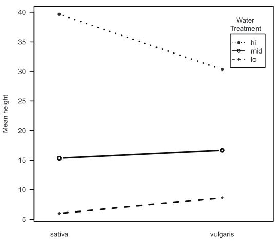
> int = interaction(pw$plant, pw$water, sep = "-")

## View the new factor > int

[1] vulgaris-lo vulgaris-lo vulgaris-lo vulgaris-mid vulgaris-mid [6] vulgaris-mid vulgaris-hi vulgaris-hi vulgaris-hi sativa-lo [11] sativa-lo sativa-lo sativa-mid sativa-mid sativa-mid [16] sativa-hi sativa-hi sativa-hi

6 Levels: sativa-hi vulgaris-hi sativa-lo vulgaris-lo ... vulgaris-mid

## Levels unordered so appear in alphabetical order > levels(int)

COMMAND NAME

rep

Creates replicated elements. Can be used for creating factor levels where replication is unequal,

for example.

Common Usage

rep(x, times, length.out, each)

Related Commands

seq

(p. 27)

gl

(p. 23)

factor

(p. 7)

interaction

(p. 24)

Command Parameters

x

A vector or other object suitable for replicating. Usually a vector, but lists, data

frames, and matrix objects can also be replicated.

times

A vector giving the number of times to repeat. If

times

is an integer, the entire

object is repeated the specified number of

times

. If

times

is a vector, it must be

the same length as the original object. Then the individual elements of the vector

specify the repeats for each element in the original.

length.out

The total length of the required result.

each

Specifies how many times each element of the original are to be repeated.

Examples

## Create vectors

> (newnum = 1:6) # create and display numeric vector [1] 1 2 3 4 5 6

> (newchar = LETTERS[1:3]) # create and display character vector [1] "A" "B" "C"

## Replicate vector

> rep(newnum) # Repeats only once [1] 1 2 3 4 5 6

> rep(newnum, times = 2) # Entire vector repeated twice [1] 1 2 3 4 5 6 1 2 3 4 5 6

THEME

1

: D

A

T

A

> rep(newnum, each = 2, length.out = 11) # Max of 11 elements [1] 1 1 2 2 3 3 4 4 5 5 6

> rep(newchar, times = 2) # Repeat entire vector twice [1] "A" "B" "C" "A" "B" "C"

> rep(newchar, times = c(1, 2, 3)) # Repeat 1st element x1, 2nd x2, 3rd x3 [1] "A" "B" "B" "C" "C" "C"

> rep(newnum, times = 1:6) # Repeat 1st element x1, 2nd x2, 3rd x3, 4th x4 etc. [1] 1 2 2 3 3 3 4 4 4 4 5 5 5 5 5 6 6 6 6 6 6

> rep(c("mow", "unmow"), times = c(5, 4)) # Create repeat "on the fly" [1] "mow" "mow" "mow" "mow" "mow" "unmow" "unmow" "unmow" "unmow"

COMMAND NAME

rbind

Adds a row to a matrix.

SEE

rbind

in “Adding to existing Data.”

COMMAND NAME

seq seq_along seq_len

These commands generate regular sequences. The

seq

command is the most flexible. The

seq_along

command is used for index values and the

seq_len

command produces simple

sequences up to the specified length.

Common Usage

seq(from = 1, to = 1, by = ((to – from)/(length.out – 1)), length.out = NULL, along.with = NULL)

seq_along(along.with)

seq_len(length.out)

Related Commands

Command Parameters

from = 1

The starting value for the sequence.

to = 1

Then ending value for the sequence.

by =

The interval to use for the sequence. The default is essentially 1.

length.out = NULL

The required length of the sequence.

along.with = NULL

Take the required length from the length of this argument.

Examples

## Simple sequence > seq(from = 1, to = 12)

[1] 1 2 3 4 5 6 7 8 9 10 11 12

## Specify max end value and interval > seq(from = 1, to = 24, by = 3) [1] 1 4 7 10 13 16 19 22

## Specify interval and max no. items rather than max value > seq(from = 1, by = 3, length.out = 6)

[1] 1 4 7 10 13 16

## seq_len creates simple sequences > seq_len(length.out = 6)

[1] 1 2 3 4 5 6

> seq_len(length.out = 8) [1] 1 2 3 4 5 6 7 8

## seq_along generates index values > seq_along(along.with = 50:40) [1] 1 2 3 4 5 6 7 8 9 10 11

> seq_along(along.with = c(4, 5, 3, 2, 7, 8, 2)) [1] 1 2 3 4 5 6 7

## Use along.with to split seq into intervals > seq(from = 1, to = 10, along.with = c(1,1,1,1)) [1] 1 4 7 10

> seq(from = 1, to = 10, along.with = c(1,1,1)) [1] 1.0 5.5 10.0

COMMAND NAME

scan

THEME

1

: D

A

T

A

SEE

scan

in “Importing Data” and

scan

in “Creating Data from the Clipboard.”

CREATING DATA FROM THE CLIPBOARD

It is possible to use the clipboard to transfer data into R; the

scan

command is designed

especially for this purpose.

COMMAND NAME

scan

This command can read data items from the keyboard, clipboard, or text file.

SEE

scan

in “Importing Data.”

ADDING TO EXISTING DATA

If you have an existing data object, you can append new data to it in various ways. You can also

amend existing data in similar ways.

COMMAND NAME

$

Allows access to parts of certain objects (for example, list and data frame objects). The

$

can

access named parts of a list and columns of a data frame.

SEE

also

$

in “selecting and sampling Data.”

Common Usage

object$element

Related Commands

[]

(p. 30)

c

(p. 22)

cbind

(p. 33)

rbind

(p. 36)

data.frame

(p. 6, 34)

unlist

(p. 105)

Command Parameters

Examples

## Create 3 vectors > mow = c(12, 15, 17, 11, 15) > unmow = c(8, 9, 7, 9) > chars = LETTERS[1:5]

## Make list

mylist = list(mow = mow, unmow = unmow)

## View an element mylist$mow

## Add new element > mylist$chars = chars

> ## Make new data frame > mydf = data.frame(mow, chars)

> ## View column (n.b. this is a factor variable) > mydf$chars

[1] A B C D E Levels: A B C D E

> ## Make new vector > newdat = 1:5

> ## Add to data frame > mydf$extra = newdat > mydf

mow chars extra 1 12 A 1 2 15 B 2 3 17 C 3 4 11 D 4 5 15 E 5

COMMAND NAME

[]

Square brackets enable sub-setting of many objects. Components are given in the brackets; for

vector or list objects a single component is given:

vector[element]

. For data frame or matrix

objects two elements are required:

matrix[row, column]

. Other objects may have more

dimen-sions. Sub-setting can extract elements or be used to add new elements to some objects (vectors

and data frames).

THEME

elements

Named elements or index number. The number of elements required depends on

the object. Vectors and list objects have one dimension. Matrix and data frame

objects have two dimensions:

[row, column]

. More complicated tables may have

three or more dimensions.

> mydf mow unmow V3 1 12 8 6 2 15 9 5 3 17 7 4 4 11 9 3 5 15 NA 2 6 99 NA 1

## Give name to set column name > mydf[, 'newdat'] = newdat

COMMAND NAME

c

Combines items. Used for many purposes including adding elements to existing data objects

(mainly vector objects).

SEE

also “Creating Data from the Keyboard.”

Common Usage

c(...)

Related Commands

$

(p. 109)

[]

(p. 30)

cbind

(p. 33)

rbind

(p. 36)

data.frame

(p. 6, 34)

Command Parameters

...

Objects to be combined.

Examples

## Make a vector > mow = c(12, 15, 17, 11) ## Add to vector > mow = c(mow, 9, 99) > mow

THEME

1

: D

A

T

A

## Make new vector > unmow = c(8, 9, 7, 9)

## Add 1 vector to another > newvec = c(mow, unmow)

## Make a data frame

> mydf = data.frame(col1 = 1:6, col2 = 7:12)

## Make vector > newvec = c(13:18)

## Combine frame and vector (makes a list) > newobj = c(mydf, newvec)

> class(newobj) [1] "list"

COMMAND NAME

cbind

Binds together objects to form new objects column-by-column. Generally used to create new

matrix objects or to add to existing matrix or data frame objects.

Common Usage

cbind(..., deparse.level = 1)

Related Commands

rbind

(p. 36)

matrix

(p. 10)

data.frame

(p. 6, 34)

[]

(p. 30)

$

(p. 109)

Command Parameters

...

Objects to be combined.

deparse.level = 1

Controls the construction of column labels (for matrix objects). If set to

1 (the default), names are created based on the names of the individual

objects. If set to 0, no names are created.

Examples

## Make two vectors (numeric) > col1 = 1:3

## Make matrix

> newmat = cbind(col1, col2)

## Make new vector > col3 = 7:9

## Add vector to matrix > cbind(newmat, col3) col1 col2 col3 [1,] 1 4 7 [2,] 2 5 8 [3,] 3 6 9

## Add vector to matrix without name > cbind(col3, newmat, deparse.level = 0) col1 col2

[1,] 7 1 4 [2,] 8 2 5 [3,] 9 3 6

## Make data frame

> newdf = data.frame(col1, col2)

## Add column to data frame > newobj = cbind(col3, newdf) > class(newobj)

[1] "data.frame"

COMMAND NAME

data.frame

Used to construct a data frame from separate objects or to add to an existing data frame.

SEE

also “types of Data.”

Common Usage

data.frame(..., row.names = NULL,

stringsAsFactors = default.stringsAsFactors())

Related Commands

THEME

1

: D

A

T

A

Command Parameters

...

Items to be used in the construction of the data frame. Can be object

names separated by commas.

row.names = NULL

Specifies which column will act as row names for the final data frame.

Can be integer or character string.

stringsAsFactors

A logical value,

TRUE

or

FALSE

. Should character values be converted to

factor

? Default is

TRUE

.

Examples

## Make two vectors > col1 = 1:3

> col2 = 4:6

## Make data frame

> newdf = data.frame(col1, col2)

## Make new vector > col3 = 7:9

## Add vector to data frame > data.frame(newdf, col3) col1 col2 col3

1 1 4 7 2 2 5 8 3 3 6 9

COMMAND NAME

matrix

A

matrix

is a two-dimensional, rectangular object with rows and columns. A matrix can contain

data of only one type (all text or all numbers). The command creates a matrix object from data or

adds to an existing matrix.

Common Usage

matrix(data = NA, nrow = 1, ncol = 1, byrow = FALSE, dimnames = NULL)

Related Commands