Is the Marginal Child More Likely to
be Murdered?
An Examination of State Abortion Ratios and
Infant Homicide
David E. Kalist
Noelle A. Molinari
a b s t r a c t
We examine whether abortion removes from the population those infants most at risk of homicide. As part of our identification strategy, we find that abortion reduces the number of unwanted births, estimating that 1 percent increase in the abortion ratio reduces unwanted births by approximately 0.35 percent. Using cross-sectional time-series data for U.S. states between 1970 and 1998, we find that an increase in the abortion ratio (a proxy for unwanted births) reduces the expected number of infant homicides, espe-cially among black infants. Overall, the elasticity of infant homicides with respect to unwanted births is approximately 0.089.
I. Introduction
This paper provides a reexamination of the adverse outcomes of the marginal child—the child that is not born due to abortion. Our research is largely motivated by the finding of Gruber, Levine, and Staiger (1999) that the marginal child is more likely to have lived in a single parent home, to have lived in poverty, to have
David E. Kalist is an assistant professor of economics at Shippensburg University. Noelle A. Molinari is a research economist affiliated with Wayne State University. The authors thank Stephen Spurr and partici-pants at the Eastern Economic Association meetings, especially Michael Grossman, for helpful comments on an early version of this paper. Address correspondence to David E. Kalist, Department of Economics, 324 Grove Hall, Old Main Drive, Shippensburg, PA, 17257-2297. Telephone: (717) 477-1437. Email: [email protected]. The data used in this article can be obtained beginning January 2007 through December 2010 from David E. Kalist, Department of Economics, 324 Grove Hall, Old Main Drive, Shippensburg, PA, 17257-2297. Telephone: (717) 477-1437. Email: [email protected].
[Submitted March 2005; accepted October 2005]
ISSN 022-166X E-ISSN 1548-8004 © 2006 by the Board of Regents of the University of Wisconsin System
received welfare, and to have died as an infant.1We concentrate on the last outcome
by examining whether abortion rates could explain the variation in infant homicides during the period 1970–98. By using cross-sectional time-series data, we are able to examine how infant homicides vary with changes in abortion ratios, while controlling for state-specific heterogeneity (state effects) and factors that might affect infant homicide over time (year effects).
Surprisingly little research has examined infant homicide. This dearth of research is not explained by a low risk of infant homicide. In fact during the first 17 years of life, the risk of homicide in the first year is greater than any other year, with the high-est risk occurring on the day of birth (Paulozzi and Sells 2002). In addition, Paulozzi and Sells find that infant homicide is the leading cause of injury death during the first year of life and the 15thleading cause of death overall.
Policy makers’ interest in the problem of infant homicide has increased in recent years. Many states, for example, have passed laws addressing the issue of infant homi-cide, specifically infant abandonment. These so-called safe-haven laws allow a mother to relinquish her new born (in general, state laws allow abandonment of infants aged between three days and 30 days old, with some extended to 90 days) at a hospital, emergency medical services provider, police or fire station, or church. These laws are designed to prevent mothers from either killing their unwanted infant or abandoning their infant in a potentially life threatening environment, such as a trash dumpster or a park bench during inclement weather. Data on infant abandonment is sparse and problematic (law enforcement only knows of the infants found), but the U.S. Department of Health and Human Services estimated that 105 infants were aban-doned in public places during 1998 and, of those, 33 were found dead. By compari-son, there were 322 infant homicides in 1998.2
Donohue and Levitt (2001) suggest that legalized abortion reduces the number of children growing up with parents, in most cases a single mother, that are unable to make sufficient investments in the child’s human capital. It is in this type of house-hold that the incidence of infant homicide is likely to be higher.
Bitler and Zavodny’s (2004) finding that legalization of abortion has reduced the inci-dence of child abuse and neglect seems to corroborate the effects of abortion legalization on child outcomes. However, they fail to find a link between abortion legalization and child deaths and murders (aged 0-17). Our methods differ in that we consider whether the rate of abortion affects the number of murders from a very narrow subset of children, namely infants. Other effects on abortion, such as the legal reforms prior to Roe v. Wade, are noted by Angrist and Evans (1999) to have reduced out-of-wedlock childbearing among teens and increased schooling especially among young black women.
In the paper, we examine whether the marginal child is at greater risk of being mur-dered. Specifically, we assume that unwanted infants, if born, would be at increased The Journal of Human Resources
612
1. Gruber, Levine, and Staiger (1993) do not examine specific causes of death but rather use infant mortality. 2. Texas is the first state to pass a safe-haven law (1999), and, by 2003, 43 states have enacted similar laws. Some states with safe-haven laws have affirmative defense in which case a parent can still be prosecuted for relinquishing the infant, but the act of leaving an infant at a safe-haven is a defense against prosecution for abandonment, abuse neglect, or child endangerment. Information on safe-haven laws is available at
http://naic.acf.hhs.gov/general/legal/statutes/safehaven.cfm#noteone. Data on infant abandonment are from
risk of homicide. We examine the variation in infant homicides (victims aged less than one year) across states and over time and test whether abortion culls from the popu-lation those infants at highest risk of infant homicide.
II. Literature Review
Although little research examines the relationship between infant homicide and abortion, a number of studies have examined the effects of abortion on infant health outcomes, such as neonatal mortality rates and low birth weights (Corman and Grossman 1985; Grossman and Jacobowitz 1981; and Joyce 1987). In general, these studies find improved birth outcomes when access to abortion is widely available. Currie, Nixon, and Cole (1995) is a notable exception; they fail to find evi-dence of a relationship between Medicaid abortion funding and birth weight. Grossman and Jacobowitz (1981) write, “The most striking finding is that the increase in the legal abortion rate is the single most important factor in reductions in both white and nonwhite neonatal mortality rates.” Overpeck et al. (1998) indicate that some of the characteristics associated with infant homicide are low birth weight, low gestational age, low Apgar3scores, and male sex.4We expect healthier infants to be less likely to
die from child abuse than unhealthy infants, such as those born with low birth weight. Furthermore, parents should be less likely to abuse a healthy infant. Because male infants are generally less healthy than females, male infants are likely to be at increased risk of dying from neglect, abandonment, or maltreatment.5
Sorenson, Weibe, and Berk (2002) is the only research we are aware of that exam-ines the link between abortion and infant homicide. They use time series data to deter-mine whether the United States Supreme Court’s 1973 decision in Roe v. Wadeleads to a subsequent decline in homicides of young children. Using 38 years of data, they find that the legalization of abortion is associated with a statistically significant reduc-tion in the number of one- to four-year-old homicide victims but has no effect on the numbers of infant homicides.6However, their approach fails to address the possibility
3. The Apgar score is a method of evaluating the health of a new born infant and is usually administered at one and five minutes after birth. The score is based on the baby’s heart rate, respiration, muscle tone, reflex response, and color. A low score, for example, could reflect a weak heart rate, limp muscle tone, poor skin color, and/ or a weak cry.
4. The result that male sex is a risk factor seems counterintuitive given that male children are preferred to female children in many cultures (see Stephen E. Landsburg, “Oh, No: It’s a Girl: Do Daughters Cause Divorce,” accessed at http://slate.msn.com/id/2089142/and Dahl and Moretti 2003). Between 1976 and 1999, 2,505 male infants were killed while only 2,201 female infants killed. It is quite possible, however, that conditional on health status males are abused at a lower rate than females (consistent with the idea that males are preferred to females), but because males are generally less healthy, they are more likely to die from abuse than females.
5. The neonatal (younger than 28 days), post-neonatal (between 28 days and 11 months), and infant mor-tality (younger than 1 year) rates are historically higher for males than females. In 2001 the male neonatal, post-neonatal, and infant mortality rates were 5.0, 2.5, and 7.5, respectively; the corresponding female rates were 4.1, 2.1, and 6.1, respectively (Centers for Disease Control and Prevention, National Vital Statistics Reports, Vol. 52, No. 3, September 18, 2003).
6. The authors also fail to control for other potentially important factors that may affect the level of infant homicides, such as the number of live births, the state of the economy, and transfer payments.
that changing societal factors may have coincided with Roe v. Wade, making it difficult to parse out the separate effects of abortion legalization on homicides. Our analysis overcomes this weakness by using cross-sectional time series data at the state level.
III. Infant Homicide: An Overview
Our data on infant homicides (victims aged less than 1 year) are from the National Vital Statistics System (NVSS), produced by the Centers for Disease Control and Prevention National Center of Health Statistics (NCHS).7The mortality
data collected by the NCHS originate from death certificates filed in each state. This collection method differs from the FBI’s Uniform Crime Reporting data or Supplemental Homicide Reports (SHR), which rely on the self reporting of state and local law enforcement agencies. Organizations involved in child welfare research, such as Child Trends, generally use NVSS data. Nevertheless, Wiersema, Lofton, and McDowell (2000) report that “empirical evidence for the equivalence of the data sources comes from studies that show close agreement between the NVSS and the SHR at large geographic scales, such as the nation or state.”
For the purposes of the NVSS, a homicide results from an injury inflicted by another person with the intent to injure or kill. It should be noted that infant homicide data have certain unique limitations. Unlike adult victims, infant victims are more eas-ily concealed. Other than the perpetrator, it is possible no one would be aware that an infant is missing or dead. Further, some infant homicides might be mistakenly attrib-uted to natural causes (for example, sudden infant death syndrome). Although it is possible that some stillbirths might be classified as homicides, the effect is likely too small to present significant upward bias of the data (Paulozzi and Sells, 2002).
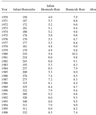
Table 1 shows national data on infant homicides, infant homicide rates (measured per 100,000 live births), homicide rates (measured per 100,000 population), and abor-tion ratios (number of aborabor-tions per 1,000 live births) between 1970 and 2000. During the period of analysis, the infant homicide rate more than doubles from 4.0 in 1970 to 8.6 in 2000. In contrast to the overall homicide rate, which fell dramatically during the 1990s, the infant homicide rate has remained relatively steady. In 2003, the infant homicide rate was 7.8, about 15 percent lower than its peak of 9.2 in 1991. Over the same period, the overall homicide rate fell more than 40 percent. There is, however, more noise in the national infant homicide rate. For example, the variation in the infant homicide rate relative to its mean (CV = 23.4 percent) is about 1.7 times that of the homicide rate (CV = 14 percent).
One might suspect that infant homicide is related to the overall level of crime in a state. Fiala and Lafree (1988) find that a cultural orientation to violence, measured using a nation’s war history, is predictive of child homicide rates. We calculate Spearman rank correlation coefficients between the state-level infant homicide rate and other crime rates. The infant homicide rate is positively correlated with the level of crime in a state, with the strongest linear correlation associated with the violent
7. The NCHS provides one of the most comprehensive sources of data pertaining to health issues in the United States.
crime rate (rho= 0.34, p< 0.01). The correlation with the overall homicide rate is slightly lower (rho= 0.21, p<0.01). In contrast, the other measures of crime (homi-cide rate, violent crime rate, and property crime rate) are much more highly correlated with one another than with the infant homicide rate. For example, the correlation between the violent crime rate and property crime rate is 0.70 (p<0.01).
Kalist and Molinari 615
Table 1
Homicide and Abortion Data
Infant
Year Infant Homicides Homicide Rate Homicide Rate Abortion Ratio
1970 150 4.0 7.9 52
1971 187 5.3 8.6 137
1972 172 5.2 9.0 180
1973 161 5.1 9.4 196
1974 166 5.2 9.8 242
1975 178 5.6 9.6 272
1976 170 5.3 8.7 312
1977 177 5.3 8.8 325
1978 161 4.8 9.0 347
1979 170 4.9 9.8 358
1980 210 5.8 10.2 359
1981 218 6.0 9.8 358
1982 243 6.6 9.1 354
1983 193 5.3 8.3 349
1984 237 6.5 7.9 364
1985 200 5.3 8.0 354
1986 278 7.4 8.5 354
1987 273 7.2 8.3 356
1988 315 8.1 8.4 352
1989 335 8.4 8.7 346
1990 332 7.9 9.4 344
1991 380 9.2 9.8 338
1992 326 8.0 9.3 334
1993 340 8.6 9.5 333
1994 313 7.9 9.0 321
1995 311 8.0 8.2 311
1996 332 8.5 7.4 315
1997 317 8.1 6.8 306
1998 322 8.2 6.3 264
1999 331 8.4 5.7 256
2000 349 8.6 5.5 245
Although we do not consider the issue in this paper, it is possible that the overall level of crime negatively influences fertility rates; some people may not wish to raise children in a violent environment. The effect on the infant homicide rate, however, is ambiguous, depending on which types of households are relatively more sensitive to violence. For example, if suburban households are more concerned about raising chil-dren in a violent world relative to urban households, the infant homicide rate should rise. However, if urban households, due to their proximity to violence, are more sen-sitive to raising children in violent environments, the result should be a lower infant homicide rate due to decreased fertility.
An important aspect of infant homicide data is its frequency distribution. Many states, for any given year, report zero infant homicides. In fact, approximately 20 per-cent of all observations during the period of analysis are zero. Because excluding states with zero infant homicides would introduce potentially serious bias, we use methods appropriate for count-data analysis, which take into account the distribution of the data and the preponderance of zeros.8
IV. Abortion and Unwantedness
One major concern regarding the hypothesized relationship between abortion and infant homicide is that abortion may not serve as an adequate proxy for the number of unwanted births avoided. One possible scenario illustrates this point. Assume that conditions are such that abortion ratios are declining. If abortion rates proxy for unwanted births avoided, this decline would imply an increase in unwanted births. This implication could be false, however, if the decline in abortion rates is due to women relying more heavily on other forms of contraception, having less sex, or using contraceptives more effectively. One criticism of Donuhue and Levitt (2001) by Joyce (2004) is that yearly fluctuations in the abortion ratio do not reflect changes in the number of unwanted births. Joyce writes:
. . . abortion is endogenous to sexual activity, contraception and fertility. Some pregnancies that were aborted in the mid- to late 1970s may not have been con-ceived had abortion remained illegal. This weakens the link between abortion and unwanted childbearing.9
Levine (2004) adds that Donuhue and Levitt’s findings are “supported only if those [middle to late 1970s] additional abortions resulted in fewer unwanted births.”
Unfortunately, there is little empirical evidence of the link between abortion and unwantedness in the literature. An indirect test of this link by Bitler and Zavodny (2002) finds that abortion legalization causes a significant decrease in adoptions (a proxy for unwanted children) of children born to white women, indicating that abortion and
8. There are three characteristics of count variables: (1) nonnegative integer values, (2) no a priori natural upper bound, and (3) the value will equal zero for some of the observations in the population (Wooldridge, p. 645, 2002).
9. Donhue and Levitt (2004) are perplexed by this argument, which implies that abortion does not affect birth outcomes, and they cite the findings of Joyce (1987) who contends that abortions prevent unwanted births and thus the health outcomes of those born are better.
unwantedness are inversely related. Their study was limited to 1961–75, so it is not clear whether abortion remains a suitable proxy for unwantedness through the 1980s and 1990s. Levine (2004) concludes that legalization in the early 1970s resulted in fewer unwanted births. Given that there is no evidence of changes in sexual activity or use of contraceptives, Levine states that, “Each additional abortion largely replaced one (pre-sumably) unwanted birth.” Here again, one might question whether these findings hold for later time periods.
To examine the relationship between the abortion ratio and unwantedness, we use a more direct test—a regression of unwanted births on the abortion ratio. A negative coefficient on the abortion ratio would give some assurance of the suitability of using abortion as a proxy for unwanted births. It may also address some of the criticisms of Donohue and Levitt (2001) by strengthening their results.
We use data on unwanted births from CDC’s Pregnancy Risk Assessment Monitoring System (PRAMS). PRAMS collects state-specific data on maternal experiences and infant health. Most importantly for our purposes, PRAMS provides information on unin-tended pregnancies. The CDC began collecting PRAMS data in 1988 for only two states. In 1993 the number of states participating in PRAMS increased to ten and, by 1999, 17 states were participating.10In 1999, the 515,210 abortions in these 17 states represent
39.2 percent of abortions nationwide. Data are currently available through 1999. We construct an unbalanced panel of state-level data for the period 1993–99. The dependent variable measures the degree of unwantedness and is either (1) the proportion of pregnancies that were unwanted at conception or at any time among women giving live birth or (2) the number of unwanted births divided by the population of women aged 15–44.11The independent variable of interest is either the abortion ratio (number of
abor-tions per 1,000 live births) or the abortion rate (the number of aborabor-tions per 1,000 women aged 15–44.12In some of the regressions, we control for state characteristics such as the
unemployment rate, income per capita, income maintenance payments per capita pay-ments, Medicaid payments per capita, population and population density. We use fixed-effects estimation and year dummy variables to control for time fixed-effects and robust standard errors, adjusted for clustering at the state level, are reported. Since the depen-dent variable is a proportion, we also estimate a generalized linear model appropriate for fractional responses, following the methods of Papke and Wooldridge (1996).13
Results are presented in Table 2 and indicate that the abortion ratio and abortion rate are negatively related to unwanted births in a state. Despite the small sample
10. The 17 states are Alabama, Alaska, Arkansas, Colorado, Florida, Illinois, Louisiana, Maine, New Mexico, New York, North Carolina, Ohio, Oklahoma, South Carolina, Utah, Washington, and West Virginia. 11. Ideally, one would prefer a measurement of unwantedness at or near birth, since attitudes regarding unwantedness may change during the course of pregnancy. It should be noted, however, that women may find it difficult to admit that their baby is unwanted after giving birth to it. The unwantedness measure is there-fore likely biased downward.
12. We use two sources for our abortion data: the Alan Guttmacher Institute and Centers for Disease Control and Prevention.
13. We use the GLM procedure in Stata (http://www.stata.com/support/faqs/stat/ logit.html). One alternative to this is to model the log odds ratio. However, as Papke and Wooldridge (1996) warn this method has short-comings: (1) the dependent variable cannot take values of 0 or 1 with a positive probability and (2) the expected value of ygiven xcannot be recovered unless one makes distributional assumptions that are not robust to distributional failure.
The Journal of Human Resources
618
Table 2
Regression Results of Abortion on Unwanted Childbearing with State Fixed-Effects, 1993–99
Dependent Variable
Proportion of Proportion of Proportion of Proportion of Unwanted births / Unwanted births /
Variable Unwanted Births Unwanted Births Unwanted Births Unwanted Births Women 15–44 Women 15–44
Abortion ratio −0.00017 −0.00017
(0.000046) (0.000092)
-0.383 -0.39483
Abortion rate −0.00250 −0.00239 −0.0001606 −0.0001437
(0.00076) (0.00154) (0.000073) (0.000138)
-0.366 -0.350 -0.367 -0.329
State controls no no yes yes no Yes
State yes yes yes yes yes Yes
fixed-effects
Year effects yes yes yes yes yes Yes
R2 0.896 0.895 0.902 0.901 0.91 0.912
Kalist and Molinari
619
AGI Data AGI w/o interpolation GLM GLM
Proportion of Proportion of Proportion of Proportion of Proportion of Proportion of
Variable Unwanted Births Unwanted Births Unwanted Births Unwanted Births Unwanted Births Unwanted Births
Abortion ratio −0.00012 −0.00008 0.00284 0.00098 −0.001841
(0.00004) (0.00007) (0.000519) (0.0018) (0.00072)
-0.323 -0.214 0.81 2.8 -0.417
Abortion rate −0.026279
(0.01235)
-0.378
State controls no yes yes yes yes yes
yes yes yes yes yes yes
fixed-effects
Year effects yes yes yes yes yes yes
Log likelihood −20.1 −20.1
R2 0.88 0.89 0.87 0.99
N 85 85 20 20 81 81
sizes, the abortion coefficients are, in many cases, precisely estimated. The estimated elasticities (which are in bold) range from −0.21 to −0.42. This is the first direct evi-dence of the relationship between abortion and unwantedness for a period far removed from the 1973 Roe v. Wadedecision. This is an important contribution to our identifi-cation strategy, since we use variations in state abortion ratios to proxy for variations in unwantedness.14 It should be noted, however, that when the abortion rate is the
covariate of interest and state controls are included, the coefficients are not statisti-cally significant except in the GLM model. When AGI data is used without interpo-lation, the effect also disappears. Given the persistence of estimates across models, it is likely that this is due to the small sample sizes.
The AGI reports that the abortion ratio increased from 193 in 1973 to a peak of 304 in 1983 (Finer and Henshaw 2003). Assuming an elasticity of unwanted births with respect to the abortion ratio of −0.35, implies that the proportion of unwanted births decreased about 20 percent over this period. Similarly, the impact of legalization of abortion caused the abortion ratio to increase from 180.1 in 1972 to 242 in 1974. This 34 percent increase may have led to approximately a 12 percent decline in the pro-portion of unwanted births, which is likely a lower bound estimate given that sexual practices were still evolving in response to the Roe v. Wade decision.
V. Abortion and Infant Homicide
As mentioned in the previous section, count data analysis is appropri-ate given the characteristics of the dependent variable. Therefore, we use negative binomial regression models to test for a relationship between abortion and infant homi-cide. Poisson models are also estimated but have a poorer fit due to over-dispersion (that is, the variance of the outcome variable exceeds its mean).15We use the
condi-tional fixed-effects negative binomial model of Hausman, Hall, and Griliches (1984) to avoid the incidental parameters problem of nonlinear panel data models. This model is estimated using Stata’s XTNBREG command with the FE option. Unfortunately, standard errors from XTNBREG cannot be adjusted for heteroskedasticity of unknown form or for within-panel correlation in errors. Therefore, we estimate unconditional negative binomial regression models (Stata’s NBREG command) with state dummy variables representing fixed-effects and standard errors adjusted for arbitrary het-eroskedasticity and arbitrary correlation across errors within a state. The tradeoff of better standard errors, of course, is that the parameter estimates are inconsistent. All fitted models include year dummy variables.
The dependent variable in our regressions is the number of infant homicides mea-sured at the state level, and separate regressions are estimated for white and black
vic-14. We also try mistimed births as a dependent variable, which measures the percent of pregnancies in which the woman wanted to be pregnant at a later time among women who gave live birth. The abortion coeffi-cients for this regression are not shown but are in all cases statistically insignificant.
15. An assumption underlying Poisson regression is that the variance and mean are equal. If there is overdis-persion, Poisson estimates are inefficient with standard errors biased downward. We calculate the deviance chi-squared statistic and reject the null hypothesis that the data are Poisson distributed. In addition, after esti-mating our negative binomial models, we reject the null hypothesis that the dispersion parameter, α, is zero. The negative binomial model equals the Poisson model when αis zero.
tims. The explanatory variables are the abortion ratio, unemployment rate, per capita income, state population, population density, fertility rate, per capita income mainte-nance payments, per capita Medicaid payments, number of police per capita, number of prisoners per capita, and natural log of live births (the exposure variable, which controls for the number of infants at risk of homicide). The primary variable of interest is the abortion ratio (the number of abortions divided by live births). Data on abortion are based on state of residence, not state of occurrence, and are from the Alan Guttmacher Institute (AGI) for the period 1970–98. These data were obtained from John Donohue’s Web site and are part of the updated abortion data used by Donuhue and Levitt (2004) in their rebuttal to Joyce (2004).16It should be noted that the AGI did not collect data
on the number of abortions in 1983, 1986, 1990, 1993, 1994, 1997, and 1998.17For
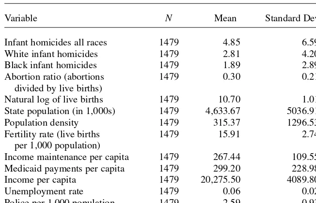
these years, the data are interpolated; however, we show results without interpolated data in the Appendix. In addition, the data from 1970–72 are backcasted from 1973 data by Donohue and Levitt (2004). Descriptive statistics are reported in Table 3.
The analysis examines two time windows. First, we examine the period 1973–98. We then extend the time window to include the pre Roe v. Wadeperiod, analyzing the period 1970–98. The benefit of adding data prior to the 1973 Roe v. Wadedecision is that a handful of states already had de facto legalized abortion: Alaska, California, Hawaii, New York, and Washington. Other states, however, allowed abortion under special circumstances such as life endangerment. Donuhue and Levitt’s data do not contain abortion data for these reform states, even though in some cases these states had higher abortion ratios. However, Donohue and Levitt (2004) state that this meas-urement error causes an attenuation of their estimates. We include a dummy variable that equals one for those states allowing abortion in special circumstances prior to 1973.18Therefore, it is likely that results presented here on the effect of abortion on
infant homicide will be biased towards zero, which is why we also present our regres-sion estimates based on the post Roe v. Wadeperiod.
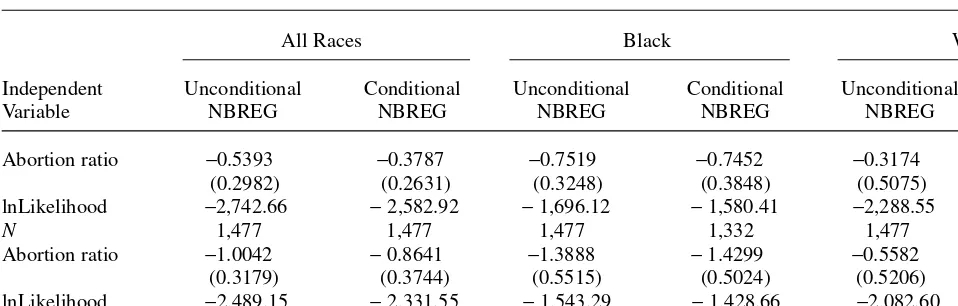
Regression results for the period 1970–98 are presented in the top half of Table 4 while results for the period 1973–98 are presented in the bottom half. The results are reported separately by race and estimation method, the fixed-effect negative binomial model and the unconditional negative binomial model. Starting with the top half of the table, the coefficient on the abortion ratio in all models is negative, indicating that in the absence of abortion the marginal child has a greater likelihood of being murdered. However, the results are only statistically significant for the regressions of black infant homicides and marginally significant for the all-races conditional regression. In terms of marginal effects (calculated from the conditional model), if the number of abortions per 1,000 live births increases by 100, black infant homicides would decrease by 5.3 percent.19 Given a one standard deviation increase in the abortion rate, black infant
homicides would decrease by 11.4 percent. The estimated elasticity (calculated at the means of the independent variables for the conditional model) is −0.023.
16.http://islandia.law.yale.edu/donohue/Abortion.htm.
17. This is from our email correspondence with Stanley Henshaw, Senior Research Associate at the AGI. 18. The twelve reform states are listed in Levine et al. (1999) and the coding used is the same as that in Angrist and Evans (1999) except that Levine et al. include Florida as a reform state. We also try the reform state coding of Bitler and Zavodny (2002); the results are essentially unchanged.
19. The 10th, 25th, 50th, 75th and 90th percentile distribution for the number of abortions per 1,000 live births are 60, 182, 300, 392, and 536, respectively.
For the period 1973–98, the coefficients on the abortion ratio are all negative, about twice as large in magnitude, and more precisely estimated. The abortion coefficients are statistically significant for the regressions on all races and black infant homicides, but remain statistically insignificant for the white infant homicide regressions. The marginal effects imply that if the number of abortions per 1,000 live births increases by 100, infant homicides will decrease for all races by 5.8 percent and for blacks by 7.6 percent. Given this finding, we estimate that an additional 20,000 abortions will prevent one infant homicide.20 The estimated abortion elasticities for the all-races
20. From a public policy perspective, if the social disutility of 20,000 abortions exceeds the social disutility of one infant homicide, than abortion is not an efficient method of preventing infant homicide.
The Journal of Human Resources 622
Table 3
Descriptive Statistics
Variable N Mean Standard Deviation
Infant homicides all races 1479 4.85 6.59
White infant homicides 1479 2.81 4.20
Black infant homicides 1479 1.89 2.89
Abortion ratio (abortions 1479 0.30 0.21
divided by live births)
Natural log of live births 1479 10.70 1.01
State population (in 1,000s) 1479 4,633.67 5036.91
Population density 1479 315.37 1296.53
Fertility rate (live births 1479 15.91 2.74
per 1,000 population)
Income maintenance per capita 1479 267.44 109.55
Medicaid payments per capita 1479 299.20 228.98
Income per capita 1479 20,275.50 4089.80
Unemployment rate 1479 0.06 0.02
Police per 1,000 population 1479 2.59 0.93
Prisoners per 1,000 population 1477 1.91 1.68
conditional regression and black conditional regression are −0.062 and −0.039, respectively.
It is interesting to note that the abortion coefficients are smaller for the regressions that include observations from the pre Roe v. Wadeperiod. As Donohue and Levitt (2004) suggest, this is the result of measurement error. States that allowed abortions only in cases of life endangerment prior to Roe v. Wadeare not treated differently in the data. In fact, if we exclude the dummy variable that indicates which states per-formed abortions only in special circumstances, the attenuation of our estimates becomes more severe.21
To estimate the effect of unwantedness on infant homicide requires combining the elasticity estimates from the homicide and unwantedness regressions. For example, if the estimated elasticity of unwantedness with respect to the abortion ratio is approxi-mately −0.35, and the elasticity of black infant homicides with respect to the abortion ratio is −0.031 (the mean of −0.023 and −0.039), then the elasticity of infant homi-cides with respect to unwantedness is 0.089. Therefore, a 10 percent increase in the percentage of unwanted pregnancies, say from 10 to 11 percent, would increase infant homicides by just under one-tenth of 1 percent.
A. Controlling for Out-of-Wedlock Births
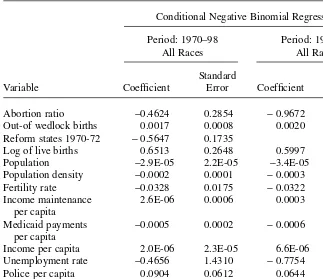
It could be argued that because change in the number of out-of-wedlock births is likely correlated with abortions and infant homicides the model should account for this. Because the data on out-of-wedlock births are incomplete for some states, espe-cially during the 1970s, we present these results separately from Table 4. Table 5 pre-sents results after controlling for out-of-wedlock births in the conditional negative binomial regression model for the periods 1970-98 and 1972-98. Including out-of-wedlock births in the black infant and white infant homicide regressions had little effect on the results, so we only show the results for all races.
The abortion coefficients are larger in magnitude than the abortion coefficients in the comparable models of Table 4. For the period 1970–98, the abortion coefficient is now statistically significant at the 10 percent level; for the period 1972–98, the abortion coefficient remains statistically significant (p = 0.015). As for out-of-wedlock births, it has a positive effect on infant homicides. A 10 percent increase in the number of out-of-wedlock births is expected to increase infant homicides by almost 1 percent.
B. Sensitivity Tests
We check the sensitivity of our results in several ways. First, we exclude Washington, D.C. from the analysis, which has had the highest abortion ratio historically, to see
21. There is reason to believe that the coefficients on the abortion ratio for the black infant homicide regres-sions are overstated because the data on abortion are not race specific. The black abortion ratio over our period of analysis is from 1.60 to approximately 2.80 times larger than the white abortion ratio, or about 1.33 to 2.0 times the overall abortion ratio. Therefore, the abortion coefficients from the black infant homicide regressions may be overstated by as much as 2.0 times. In contrast, the abortion coefficients from the white infant homicide regressions may need to be adjusted upwards from 34 to 58 percent, since the white abor-tion rate is between 0.65 and 0.75 times the overall aborabor-tion ratio.
The Journal of Human Resources
624
Table 4
Infant Homicide: Negative Binomial Regression (NBREG)
All Races Black White
Independent Unconditional Conditional Unconditional Conditional Unconditional Conditional
Variable NBREG NBREG NBREG NBREG NBREG NBREG
Abortion ratio −0.5393 −0.3787 −0.7519 −0.7452 −0.3174 −0.3219
(0.2982) (0.2631) (0.3248) (0.3848) (0.5075) (0.4061)
lnLikelihood −2,742.66 −2,582.92 −1,696.12 −1,580.41 −2,288.55 −2,144.56
N 1,477 1,477 1,477 1,332 1,477 1,477
Abortion ratio −1.0042 −0.8641 −1.3888 −1.4299 −0.5582 −0.5568
(0.3179) (0.3744) (0.5515) (0.5024) (0.5206) (0.5661)
lnLikelihood −2,489.15 −2,331.55 −1,543.29 −1,428.66 −2,082.60 −1,940.44
N 1,326 1,326 1,326 1,196 1,326 1,326
whether this small area was unduly affecting our results. The results are virtually unchanged from this exclusion. Next, we exclude both Washington, D.C. and Hawaii (a small state with a fairly high abortion ratio over the period of analysis) and find the results are robust. There is always concern about potential omitted variable bias, and one such factor over the period of analysis might be the crack cocaine epidemic that started in the mid-1980s. Therefore, we restrict our regressions to the period
Kalist and Molinari 625
Table 5
The Effects of Abortion and Out-of-Wedlock Births on Infant Homicide
Conditional Negative Binomial Regression
Period: 1970–98 Period: 1973–98
All Races All Races
Standard Standard
Variable Coefficient Error Coefficient Error
Abortion ratio −0.4624 0.2854 −0.9672 0.3967
Out-of wedlock births 0.0017 0.0008 0.0020 0.0008
Reform states 1970-72 −0.5647 0.1735
Log of live births 0.6513 0.2648 0.5997 0.2993
Population −2.9E-05 2.2E-05 −3.4E-05 2.4E-05
Population density −0.0002 0.0001 −0.0003 0.0002
Fertility rate −0.0328 0.0175 −0.0322 0.0188
Income maintenance 2.6E-06 0.0006 0.0003 0.0006
per capita
Medicaid payments −0.0005 0.0002 −0.0006 0.0002
per capita
Income per capita 2.0E-06 2.3E-05 6.6E-06 2.4E-05
Unemployment rate −0.4656 1.4310 −0.7754 1.4591
Police per capita 0.0904 0.0612 0.0644 0.0629
Prisoners per capita −0.0303 0.0283 −0.0498 0.0304
lnLikelihood −2,355.54 −2,165.36
N 1,360 1,244
preceding the epidemic, 1973–84. The coefficients on the abortion ratio remain neg-ative and statistically significant, especially for the regressions using infant homicides for all races. Moreover, the newly constructed crack-cocaine index of Fryer et al. (2005) allows us to check the sensitivity of our results over the period of the crack epi-demic. The state-specific crack index is used as an independent variable in our regres-sions on infant homicides for the period 1980–98.22The correlation between the crack
index and the number of infant homicides is 0.28. Although the coefficient on the crack index is found to be statistically insignificant in these regressions,23the
coeffi-cient on the abortion ratio is negative and statistically significant (p< 0.10). From the conditional negative binomial regression model, the elasticity of black infant homi-cides with respect to the abortion ratio is −0.091 (standard error = 0.0496) and the elasticity of infant homicides (all races) with respect to the abortion ratio is −0.052 (standard error = 0.0346).
For a final specification test, we replace the dependent variables in Table 4 with the number of homicides of children 5 to 9 years of age by race.24We expect that the
number of contemporaneous abortions should have no effect on the homicides of young children, and our results confirm this. In 11 out of the 12 regressions, the coef-ficient on abortion (which was positive in many cases) was statistically insignificant. In the one regression (unconditional NBREG for Whites, 1970–98) for which the coefficient was statistically significant (p= 0.062), it is positive.
Because the abortion ratio serves as a proxy for unwantedness in our infant homi-cide regressions, we regress infant homihomi-cides on the proportion of unwanted births, along with a number of covariates that control for state characteristics, including year and state fixed-effects. We expected to find a positive relationship between the vari-ables. However, the results of the conditional negative binomial regression results failed to find a statistically significant effect of unwantedness on infant homicide. The coefficient on unwantedness in the white infant homicide regression was positive (5.09) but statistically insignificant (p= 0.51). The coefficient on unwantedness in the black infant homicide regression was negative (−2.75) but also statistically insignifi-cant (p= 0.753). The imprecise parameter estimates are likely the result of the small sample sizes (Nranged from 72 to 79) attributable to the limited data on unwanted births. Nevertheless, failure to find a statistically significant relationship from this direct test of homicide on unwantedness should be considered in light of the findings in the remainder of the paper.
22. The crack index is available at Ronald Fryer’s faculty Web page (http://post.economics.harvard.edu/ faculty/fryer/fryer.html). We used the state-level crack index and the crack index adjusted for racial compo-sition, but the results were virtually unchanged. Fryer et al. (2005) report that the relationship between crack and adverse social outcomes diminished by the early 1990s. Therefore, we reestimated our regressions over the 1980-91 period. The estimated abortion coefficient in the all infants regression loses some precision but remains statistically significant (p< 0.10). For the regression using black infant homicides, the coefficient on abortion ratio is also measured with less precision and is not statistically significant (p= 0.16). 23. However, the crack index was positive and highly significant in regressions without fixed-effects and year dummies.
24. The data on the number of homicides of children 5 to 9 have the characteristics of count data. More than 25 percent of the state-year observations report zero homicides. The mean number of homicides per state is 3.06 (standard deviation = 4.23) for the period 1970-98. These data are also from the NVSS.
VI. Conclusion
In this paper, we are primarily interested in examining the relationship between abortion and infant homicide. We provide evidence that abortion reduces unwanted births by examining the relationship between the percent of unwanted births and the abortion ratio at the state level. We estimate that a 10 percent increase in the abortion ratio reduces unwanted births by approximately 3.5 percent. With this finding, we have evidence that the abortion ratio is a suitable proxy for unwantedness in our infant homicide regressions.
The results from the infant homicide regressions suggest that higher abortion ratios are associated with fewer infant homicides. These results are consistent with previous research on the marginal child, which indicates that abortion culls from the popula-tion those infants most at risk of living in undesirable condipopula-tions. The results are robust across different specifications, time periods, and estimation techniques, such as conditional and unconditional negative binomial regression models. These results remain robust even after controlling for the crack cocaine epidemic by using a newly created crack index. Combining the elasticity estimates from the unwantedness regressions with those from the infant homicide regressions implies that the elasticity of infant homicide with respect to unwantedness is 0.089.
The results suggest that policies aimed at eliminating abortion restrictions (Medicaid abortion funding restrictions, restricting private insurance coverage of abortion, requir-ing parental involvement in minors’ abortions, and mandatory waitrequir-ing periods and counseling for abortion) may have a negative effect on infant homicide. However, the tradeoff between abortions and fewer infant homicides should be considered from both public policy and public health perspectives. Specifically, we estimate that an additional 20,000 abortions would lead to one less infant homicide. There are clearly other, more effective and less invasive methods of preventing infant homicide, such as improved access to contraceptives and educational programs.
The Journal of Human Resources
628
Appendix 1
Infant Homicide: Negative Binomial Regression (NBREG) without Interpolated Data
All Races Black White
Unconditional Conditional Unconditional Conditional Unconditional Conditional
Independent Variable NBREG NBREG NBREG NBREG NBREG NBREG
I. Period of Analysis: 1970–98
Abortion ratio −0.4648 −0.2822 −0.7452 −0.6804 −0.2846 −0.3512
(0.3705) (0.2949) (0.3379) (0.4688) (0.5279) (0.4684)
logLikelihood −1,928.67 −1,779.61 −1,171.91 −1,066.42 −1,604.14 −14,70.67
Observations 1,069 1,069 1,069 943 1,069 1,048
II. Period of Analysis: 1973–98
Abortion ratio −0.9344 −0.7288 −1.538 −1.467 −.03492 −0.4908
(0.4068) (0.4341) (0.4327) (0.6123) (0.7163) (0.7064)
loglikelihood −1,676.59 −1,530.46 −1,020.35 −916.98 −1,400.04 −1,269.13
Observations 918 918 918 810 918 900
Kalist and Molinari 629
References
Angrist, Joshua, and William N. Evans. 1999. “Schooling and Labor Market Consequences of the 1970 State Abortion Reforms,” Research in Labor Economics18, S. Polachek, ed, Greenwich: JAI Press.
Bitler, Marianne P., and Madeline Zavodny. 2002. “Did Abortion Legalization Reduce the Number of Unwanted Children? Evidence from Adoptions.” Perspectives on Sexual and Reproductive Health34(1):25–33.
———. 2004. “Child Maltreatment, Abortion Availability, and Economic Conditions.”
Review of Economics of the Household2(2):119–41.
Centers for Disease Control and Prevention. 2003. National Vital Statistics Reports52(3), September 18.
Corman, Hope, and Michael Grossman. 1985. “Determinants of Neonatal Mortality Rates in the U.S.” Journal of Health Economics4(3):213–36
Currie, Janet, Lucia Nixon, and Nancy Cole. 1995. “Restrictions on Medicaid Funding of Abortion.” Journal of Human Resources31(1):159–88.
Dahl, Gordon B., and Enrico Moretti. 2004. “The Demand for Sons: The Evidence from Divorce, Fertility, and Shotgun Marriage.” NBER Working Paper No. 10281.
Donohue, John J., and Steven D. Levitt. 2004. “Further Evidence that Legalized Abortion Lowered Crime: A Reply to Joyce.” Journal of Human Resources39(1):29–49.
Donohue, John J., and Steven D. Levitt. 2001. “The Impact of Legalized Abortion on Crime.”
Quarterly Journal of Economics116(2):379–420.
Fiala, Robert, and Gary LaFree. 1988. “Cross-National Determinants of Child Homicide.”
American Sociological Review53(3):432–45.
Finer, Lawrence B., and Stanley K. Henshaw. 2003. “Abortion Incidence and Services in the United States in 2000.” Perspectives on Sexual Reproductive Health35(1):6–15.
Fryer, Ronald G., Paul S. Heaton, Steven D. Levitt, and Kevin M. Murphy. 2005. “Measuring the Impact of Crack Cocaine.” NBER Working Paper 11318 Cambridge, Mass.: National Bureau of Economic Research.
Grossman, Michael, and Steven Jacobowitz. 1981. “Variations in Infant Mortality Rates among Counties of the United States: The Role of Public Policies and Programs.”
Demography18(4):695–713.
Gruber, Jonathan, Phillip B. Levine, and Douglas Staiger. 1999. “Abortion Legalization and Child Living Circumstances: Who Is the Marginal Child?” Quarterly Journal of Economics
114(1):263–91.
Hausman, Jerry, Bronwyn H. Hall, and Zvi Griliches. 1984. “Econometric Models for Count Data with an Application to the Patents-R&D Relationship.” Econometrica52(4):909–38 Joyce, Theodore. 1987. “The Impact of Induced Abortion on Black and White Birth
Outcomes in the United States.” Demography24(2):229–44.
Joyce, Theodore. 2004. “Did Legalized Abortion Lower Crime?” Journal of Human Resources39(1):1–28.
Landsburg, Stephen E. 2003. “Oh, No: It’s a Girl! Do Daughters Cause Divorce?” Slate,
October 2, http://slate.msn.com/id/2089142/.
Levine, Phillip B., Douglas Staiger, Thomas Kane, and David J. Zimmerman. 1999. “Roe v. Wade and American Fertility.” American Journal of Public Health89(2): 199–203. Levine, Phillip B. 2004. Sex and Consequences: Abortion, Public Policy, and the Economics
of Fertility. Princeton, N.J.: Princeton University Press.
The Journal of Human Resources 630
Papke, Leslie E., and Jeffery M. Wooldridge. 1996. “Econometric Methods for Fractional Response Variables with an Application to 401 (K) Plan Participation Rates.” Journal of Applied Econometrics11(6):619–32.
Paulozzi L, and M Sells. 2002. “Variation in Homicide Risk During Infancy.” Morbidity and Mortality Weekly Report51(109):187–90.
Sorenson, Susan B., Douglas J. Wiebe, and Richard A. Berk. 2001. “Legalized Abortion and the Homicide of Young Children: An Empirical Investigation.” Analyses of Social Issues and Public Policy239–56.
Wiersema, Brian, Colin Lofton, and David McDowell. 2000. “A Comparison of
Supplementary Homicide Reports and National Vital Statistics System Homicide Estimates for U.S. Counties.” Homicide Studies4(4):317–40.