Material modeling of biofilm mechanical

Material modeling of biofilm mechanical properties

C.S. Laspidou

a,⇑

_{, L.A. Spyrou}

b

_{, N. Aravas}

c,d

_{, B.E. Rittmann}

e a

Department of Civil Engineering, University of Thessaly, Pedion Areos, 38334 Volos, Greece b

Institute for Research & Technology—Thessaly, Center for Research & Technology Hellas (CERTH), 95 Dimitriados Str., 38333 Volos, Greece c

Department of Mechanical Engineering, University of Thessaly, Pedion Areos, 38334 Volos, Greece d

International Institute for Carbon Neutral Energy Research (WPI-I2

CNER), Kyushu University, 744 Moto-oka, Nishi-ku, Fukuoka 819-0395, Japan e

Swette Center for Environmental Biotechnology, Biodesign Institute at Arizona State University, 1000 S. McAllister Ave., P.O. Box 875701, Tempe, AZ 85287-5701, USA

a r t i c l e

i n f o

Article history:

Received 13 June 2013

Received in revised form 12 October 2013 Accepted 11 February 2014

Available online 20 February 2014

Keywords:

Biofilm modeling Composite Young’s modulus Biofilm mechanical properties Consolidation

a b s t r a c t

A biofilm material model and a procedure for numerical integration are developed in this article. They enable calculation of a composite Young’s modulus that varies in the biofilm and evolves with deforma-tion. The biofilm-material model makes it possible to introduce a modeling example, produced by the Unified Multi-Component Cellular Automaton model, into the general-purpose finite-element code ABAQUS. Compressive, tensile, and shear loads are imposed, and the way the biofilm mechanical proper-ties evolve is assessed. Results show that the local values of Young’s modulus increase under compressive loading, since compression results in the voids ‘‘closing,’’ thus making the material stiffer. For the opposite reason, biofilm stiffness decreases when tensile loads are imposed. Furthermore, the biofilm is more compliant in shear than in compression or tension due to the how the elastic shear modulus relates to Young’s modulus.

Ó_{2014 Elsevier Inc. All rights reserved.}

1. Introduction

A biofilm consists of microbial cells attached to a solid surface and embedded in a matrix of organic polymers produced by cells, the extracellular polymeric substances (EPS) [19]. Biofilms are found everywhere in nature and could be detrimental when accumulating on medical implants (causing infections) or on water treatment membranes causing biofouling. They also can be benefi-cial, as in biofilm wastewater treatment processes, bioremediation systems, and microbial fuel cells [15]. Whether the goal is to encourage or discourage biofilm accumulation, detachment is one of the key determinants of how much biofilm accumulates. Although far from well understood, biofilm detachment and its correlation to biofilm mechanical properties are indisputably important[17,23,9,14,2]. Such properties include Young’s modulus and failure strength that, although routinely measured for structural materials such as steel, are not reported consistently for biofilms, as no standard measurement method exists for this material. Several researchers have made attempts to experimen-tally quantify biofilm mechanical properties, presenting a wide range of values and methodologies [7,18,20,21,16,1]. Biofilm modelers also have addressed biofilm mechanical properties and detachment[8,10,23,6].

Biofilm models based on cellular automata (CA), such as the Unified Multi-Component Cellular Automaton (UMCCA) model, represent solutes in a continuous field by reaction–diffusion mass balances and map solids in a discrete cell-by-cell fashion that em-ploys a CA algorithm [13]. In particular, UMCCA includes eight variables: active biomass (Xa), extracellular polymers, or bound EPS (EPS), residual inert biomass (Xres), pores, original donor sub-strate (S), two metabolic products, the sum of which is referred to as Soluble Microbial Products (SMP), or soluble EPS—the utiliza-tion-associated products (UAP) and the biomass-associated prod-ucts (BAP)—and oxygen. One of UMCCA’s objectives is to describe quantitatively the heterogeneity of biofilms; it calculates a variable ‘‘composite biofilm density,’’ i.e., a density that corresponds to a to-tal solids or other dry weight measurement. To explain differences in density that have also been observed experimentally [24], UMCCA includes a consolidation module that allows biofilms to become more compact as they age; it simulates correctly— according to the experimental data shown in Zhang and Bishop

[24]—that mature biofilms have bottom layers having higher den-sities than their ‘‘fluffy’’ top layers, as the bottom layers undergo consolidation for the longest time.

In this article, we develop a biofilm-material model and a procedure for its numerical implementation, and we apply the homogenization technique described in Laspidou and Aravas [9]

to calculate the local values of the elastic moduli throughout the biofilm column; biofilm modeling samples are produced with the

http://dx.doi.org/10.1016/j.mbs.2014.02.007 0025-5564/Ó2014 Elsevier Inc. All rights reserved.

⇑ Corresponding author. Tel.: +30 24210 74147; fax: +30 24210 74169.

E-mail address:laspidou@uth.gr(C.S. Laspidou).

Contents lists available atScienceDirect

Mathematical Biosciences

UMCCA model[11,12]. We use the general-purpose finite-element software ABAQUS to place the sample under tension, compression, or shear. We also map how stress and mechanical properties vary throughout the biofilm column. Finally, we assess how the explicit incorporation of consolidation makes a difference in how biofilm mechanical properties evolve.

2. Methods

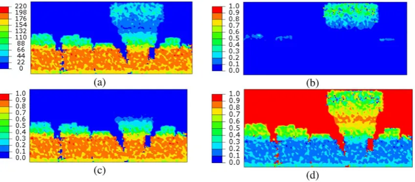
Fig. 1(a) shows a 2-dimensional biofilm-modeling example that is an output of the UMCCA model[13]. The domain is 600

l

m long and 280

l

m deep. From a solid substratum at the bottom, the biofilm develops into a ‘‘mushroom’’ shape due to the conditions imposed in the example. The key condition causing the heteroge-neous ‘‘mushrooming’’ was substrate mass-transport resistance from the bulk liquid at the top. The bottom of the biofilm, which is over 200 days old in the simulation, has the highest density values (as high as 220 g CODx/l), and the top part of the large mushroom has much lower values. To illustrate the trends for the various components of the biofilm, we present volume frac-tions forXa, Xres, and porosity inFig. 1(b) through (d), respectively. The high values of total biomass density at the bottom of the bio-film are a result of consolidation, and almost zero voids are present in the old biofilm, which had almost 200 days to consolidate. In addition, the bottom of the biofilm has very low active biomass,

Xa, since the active biomass is mostly decayed to inert residual biomass (Xres) by 200 days. The trend is similar forEPS, which is almost completely hydrolyzed at the bottom.Fig. 1makes it clear that biofilm properties can change drastically from one point to another inside the matrix, bringing about corresponding variations in biofilm mechanical properties[9,14].

Porosity plays a key role in determining the mechanical proper-ties of a porous material such as the biofilm: deformation of the biofilm changes the volume of the void space and this affects in turn the mechanical properties of the biofilm. Changes in porosity bring about changes in the volume fractions of all phases through-out the biofilm column. Thus, mechanical properties depend on volume fractions of the four phases, and the volume fractions can be altered when the biofilm deforms. A theory that quantifies deformation-dependent changes in the mechanical properties of a composite porous material, such as biofilm, was presented by Laspidou and Aravas[9].

In developing the biofilm-material model, we treat the biofilm as a four-phase composite continuum. The four phases correspond

to the three solid biomass phases (1—active biomassXa), extracel-lular polymers (2—EPS) and residual inert biomass (3—Xres)), and void space(4). Letci(i= 1, 2, 3, 4) be the volume fractions of the four phases (c1+c2+c3+c4= 1). As the biofilm deforms, the volume fractionscievolve due to the change of volume of the void space. The spatial distribution of each phase is, in general, non-uniform in a biofilm. The profiles shown inFig. 1(b) through (d) correspond to the initial values of the volume fractionsci.

Each of the four material phases is modeled as an isotropic linearly elastic material with Young’s modulus Ei and Poisson’s ratio

m

i; the Young’s modulus of the ‘‘void material’’ is negligible, i.e.,E4= 0. The voids are assumed to be initially spherical on the average and to remain spherical as the material deforms, so that overall isotropy is maintained. The biofilm is assumed to be macroscopically isotropic and a homogenization scheme is used to estimate the ‘‘effective’’ elastic properties (Ehom,

m

hom) of the homogenized isotropic composite material[22]:

Ghom¼

P4

i¼1

ciGi

6Giðj~þ2~GÞþG~ð9~jþ8G~Þ

P4 j¼1

cj

6Gjðj~þ2~GÞþG~ð9~jþ8G~Þ

j

hom¼ P4

i¼1

ciji

3jiþ4G~

P4 j¼1

cj

3jiþ4G~

ð1Þ

Ehom¼ 9Ghom

j

hom 3

j

homþGhom

m

hom¼

3

j

hom2Ghom

2ð3

j

homþGhomÞ ð

2Þ

In Eq.(1),Gi¼2ð1þEimiÞand

j

i¼

Ei

3ð12miÞare the elastic shear and bulk

moduli, respectively of the constituent phases. The valuesG~¼G2 and

j

~¼

j

2 are used in (1), since EPS is the ‘‘matrix’’ phase[4]. The values E1¼10 Pa, E2¼60 Pa, E3¼240 Pa, E4= 0 and

m

1=

m

2=

m

3= 0.45 are used in the calculations. A justification for the choice of these values appears in Laspidou and Aravas[9]. The volume fractions are position-dependent in the biofilm. Therefore, the homogenization scheme of Eqs.(1) and (2)is used at every point of the continuum in order to estimate the local values of

(Ghom,

j

hom) and (Ehom,

m

hom). Homogenization methods provide a

means of estimating the macroscopic behavior of composite-heterogeneous materials by making use of the available statistical information about their microstructure (i.e., volume fractions and spatial distribution of phases). These methods have as a purpose to link the macroscopic with the microscopic scale in the most effi-cient manner by including as much information as it is available about the microstructure of the material. In layman’s terms, in order to calculate the mechanical properties of a composite mate-rial, we cannot simply take a linear combination of the mechanical properties of the constituent phases multiplying each phase

Fig. 1.Contours of (a) biofilm density in g CODx/l; (b) volume fractionc1of active biomass before deformation; (c) volume fractionc3of residual inert biomass profile before

property by its volume fraction; we need to use Eqs.(1) and (2)to calculate the compositeEand

m

(Ehom,

m

hom).

In uniaxial tension, the constitutive equation is written in incre-mental form as

d

r

¼Ehomd

e

ð3Þ

whered

r

anddeare the stress and strain increments, and the mod-ulusEhomdepends on the volume fractionsci, which evolve as the uniaxial strainechanges. The corresponding three-dimensional ver-sion of the constitutive law is the standard hypoelastic form:

r

r ¼Le

hom:D or

r

ij r

¼ ðLe

homÞijpqDpq ð4Þ

where the summation convention on repeated Latin indices is used (Einstein notation),

r

_{is the true (Cauchy) stress tensor,}

r

r

¼

r

_ _þ

r

WW

r

is the Jaumann or co-rotational stress rate, DandWare the deformation rate and spin tensors defined as the symmetric and anti-symmetric parts of the spatial velocity gradi-ent, andLe

hom is the fourth-order isotropic elasticity tensor of the homogenized medium

ðLe

homÞijkl¼GhomðdikdjlþdildjkÞ þ

j

hom

2 3Ghom

dijdkl ð5Þ

anddijis the Kronecker delta.

The evolution of the volume fractions ci is accounted for by using the methodology described in Laspidou and Aravas[9]:

_

ci¼ ci

e

_v and c4_ ¼ ðc1_ þc2_ þc3_ Þ ð6Þ

where

e

_v¼trDis the rate of the volumetric strainev, and tr denotes

the trace of a tensor.

We implemented the biofilm-material model in the general-purpose finite-element program ABAQUS. This code provides a general interface so that a particular constitutive model can be introduced as a ‘‘user subroutine’’ (UMAT). Integration of all equa-tions involved was carried out using the algorithm presented in the

Appendix A. We used a ‘‘large strain’’ formulation, i.e., we accounted for geometric non-linearities. The finite-element formu-lation was based on the weak form of the momentum balance; the solution was carried out incrementally, and the discretized nonlinear equations were solved in ABAQUS by using Newton’s method. The Jacobian of the equilibrium Newton-loop required the so-called ‘‘linearization moduli’’ of the algorithm, which relate the variation of stress to the variation of strain over the increment.

3. Results and discussion

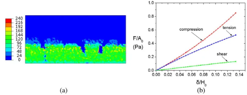
Variations in biofilm density play an important role in biofilm mechanical properties. To assess the mechanical properties of a biofilm sample, we used the volume fractions of the sample, along with the homogenization technique presented in Laspidou and Aravas[9], to calculate the elastic moduli for each modeling com-partment. Fig. 2(a) shows the spatial distribution of the initial Young’s modulusEhomin the biofilm; the local values ofEhomare higher at the bottom of the biofilm—where inert biomass is high—and the values are consistent with the graphs shown in

Fig. 1. Specifically,Fig. 1(c) shows a plot of inert biomass and we can see that at the bottom, volume fractions of inert biomass range between 0.7 and 0.8. The rest is void space (as can seen inFig. 1(d)), since active biomass and EPS are practically zero at the bottom (Fig. 1(b)). Due to homogenization, the obtained values may appear ‘‘lower than expected,’’ but are correct. This is why this type of analysis is valuable: it provides realistic values for the biofilm mechanical properties that are not easy to predict and may give prominence to critical points in the biofilm that we would or would not expect to find.

We consider a biofilm with orthogonal cross-section, as shown in Figs. 1 and 2. The initial height of the cross-section is

H0= 280

l

m and the initial width B0= 600

l

m. The length L of the biofilm in the third direction (normal to the page) is assumed to be much larger thanH0so that plane-strain conditions can be as-sumed. The biofilm is deformed in compression, tension, or shear. In the first two cases (compression or tension), a uniform vertical displacementdis imposed on the top surface of the biofilm, and the corresponding vertical forceFis calculated. In the shear prob-lem, a uniform horizontal displacementdis imposed on the top of the biofilm, and the horizontal forceFis determined. The bottom of the biofilm is constrained, and the two vertical surfaces are kept traction-free. A total of 10,200 (15068) 4-node isoparametric plane-strain elements and 20,839 degrees of freedom are used in the calculations.

Fig. 2(b) shows the normalized force–displacement curves for the three cases analyzed. In particular,Fig. 2(b) showsF=ðB0LÞvs.

d/H0. Using the so-called ‘‘mean stress’’ and ‘‘mean strain’’

theo-rems, we can readily show that F=ðB0LÞequals the average axial or shear stress in the biofilm, whereasd/H0equals the average axial or shear strain (e.g.[5], pp. 38 and 62). An important observation is that the slopes of the curves shown for tension and compression are not constant, because the local volume fractions of constituent phases evolve as the material deforms. In fact, theFdcurve is concave in tension and convex in compression. This difference is

Fig. 2.(a) Young’s modulus profiles (values in Pa); (b) normalized force–displacement curves for biofilm analyzed under compression, tension, and shear;A0=B0Lis the area

due to the change of porosity with deformation. In the tensile test, the void space increases and the material softens, whereas voids close in compression, causing the material to harden.

Even though the biofilm has high local Young’s modulus values closer to the substratum, it is not very stiff overall. This is mainly due to the empty space occupied by the fluid surrounding the mushroom cluster, which has a large percentage of empty space (zero stiffness). Also, most of the deformation happens on the top layers that have, for the most part, almost zero inerts and lower local Young’s modulus values.

The force–displacement curve in the shear test is almost linear. This is a consequence of the fact that shear deformation is volume preserving. In shear deformation, the spatial velocity gradientDis almost traceless locally, meaning thatc_i¼ citrDffi0 everywhere in the biofilm. Therefore, the volume fractions change very little from their initial local values everywhere in the biofilm, and this means that the local elastic moduli of the homogenized continuum do not change as the biofilm deforms in shear. This implies, in turn, that the overall load–displacement curve is almost linear. It should be noted also that the pores are assumed to be spherical on the average in the biofilm, thus resulting in macroscopic isotropy. Dur-ing shear deformation, the pores retain their volume, but change their shape to approximately ellipsoidal. When the void volume fractionc4is substantial and shear strains are large, the change of the void-shape may invalidate the assumption of biofilm isotropy (e.g.[3]).

Another interesting feature of Fig. 2(b) is the fact that the biofilm is more compliant (softer) in shear than in tension or com-pression. The elastic shear modulusGiin each phase is related to the corresponding Young’s modulus through a relationship of the form:

Gi¼

Ei 2ð1þ

m

iÞ

The shear modulus relates the increment of shear stressd

s

to the corresponding increment of shear strain d

c

ðd

s

¼Gid

c

Þ, whereas Young’s modulus relatesd

r

todein a uniaxial testðd

r

¼Eid

e

Þ. Since

m

i= 0.45 in all solid phases, we conclude thatGiffiE3i, i.e., all solid phases are more compliant in shear than in tension or compression. Therefore, the overall elastic behavior of the biofilm is also stiffer in tension or compression compared to shear.

Finally,Fig. 2(b) shows that the same amount of biofilm tensile, compressive or shear stress results in shear strain that is always higher than the corresponding axial strain. For example, if stress equal to 0.1 Pa is applied in compression, tension, or shear, the resultingshearstrain is about 4 times greater than the corresponding

tensileorcompressivestrain. Thus, if we assume that at the same time, axial and shear loads of equal magnitude are applied, the bio-film would be more susceptible to detachment due to shear loadings.

4. Conclusions

We develop a constitutive model for biofilms and a methodol-ogy for the numerical implementation of the model in a general-purpose finite element program; we provide also a methodology for the calculation of the local values of the elastic moduli in every modeling compartment of a biofilm produced by the UMCCA model. We show that, as the volume fractions of the biofilm solid components and voids change in the deforming biofilm, the elastic modulus evolves in a corresponding manner. Biofilm consolidation, which is included in the UMCCA model, plays an important role in biofilm mechanical properties, making old and consolidated biofilms stiffer overall, mainly due to their almost zero porosity at their bottom layers. As we impose compressive or tensile deformations on the biofilm and monitor how its mechanical

properties evolve with deformation, we show that load–displace-ment curves are non-linear and that the elastic moduli vary throughout the biofilm column. However, the load–deflection curve is linear in shear because the volume fractions change little due to shear deformation. The overall Young’s modulus of the biofilm in-creases due to voids closure when compressive loads are applied; the opposite behavior is observed in tension, since the void space increases in a tensile field. Furthermore, the biofilm is more com-pliant in shear than in tension/compression due to the inherent relationship of the elastic shear modulus to the Young’s modulus.

Acknowledgments

This work was supported by the project SOFON, which is imple-mented under the ‘‘ARISTEIA’’ Action of the Operational Pro-gramme ‘‘Education and Lifelong Learning’’ and is co-funded by the European Social Fund (ESF) and National Resources.

Appendix A

We present the methodology for the numerical implementation of the biofilm’s constitutive equations in the context of the finite element method. Standard linear isotropic hypoelasticity is used to describe the constitutive equation of the homogenized material:

r

The evolution of the volume fractions of the constituent phases is defined by

_

ci¼ ci

e

_v and c4_ ¼ ðc1_ þc2_ þc3_ Þ ð9Þ

In a finite-element environment, the solution is developed incrementally, and the constitutive equations are integrated at the element Gauss integration points. In a displacement-based fi-nite-element formulation, the solution is deformation driven. Let Fdenote the deformation gradient tensor. At a given Gauss point, the solutionðFn;

r

n;cijnÞat timetn, as well as the deformation gra-dientFn+1at timetn+1=tn+Dt, are known, and the problem is to determineð

r

_nþ1;c_ij

nþ1Þat timetn+1.

The time variation of the deformation gradient Fduring the time increment [tn,tn+1] can be written as:

FðtÞ ¼

D

FðtÞ Fn¼RðtÞ UðtÞ Fn ðtn6t6tnþ1Þ ð10Þ

whereR(t) andU(t) are the rotation and right stretch tensors asso-ciated withDF(t). The corresponding deformation rate tensorD(t) and spin tensorW(t) can be written as:

D

Fn¼Rn¼Un¼d

r

^_n¼

r

_n and

e

_n¼0 ð14Þ

whereas at the end of the increment (t=tn+1):

D

Fnþ1¼Fnþ1Fn1¼Rnþ1Unþ1¼known and

e

_{nþ1¼lnUnþ1¼known: ð15Þ}

Then, the elastic constitutive relation can be written in the follow-ing form for the time intervaltn6t6tnþ1:

_^

r

_¼Le

hom: _

e

ð16Þ

In view of (11a), we have also that

e

_v¼trD¼tr

r

_, so that the volu-metric strain associated with the increment is

D

e

v¼tr

e

nþ1¼known

where we took into account thate_n=0. The evolution equations of

the volume fractions(9)are integrated exactly to yield:

cijnþ1¼ cijneDev and

c4jnþ1¼1 ðc1jnþ1þc2jnþ1þc3jnþ1Þ ð17Þ

Eq. (16) is integrated numerically by using a central difference scheme:

^

r

_nþ1¼

r

_nþL_:

e

_nþ1; with

L ¼1

2 L

e

homðcijnÞ þ L e

homðcijnþ1Þ

ð18Þ

where we take into account that

r

^_n¼

r

_nande_n=0. Finally, the true

stress tensor

r

_n+1is computed from

r

_j

nþ1¼Rnþ1

r

^_j nþ1R

T

nþ1, which completes the integration process.

The ‘‘linearization moduli’’ of the algorithm @r_n þ1

@enþ1 are approxi-mated by

@

r

_nþ1 @

e

_nþ1ffi

L_¼1

2½L e

homðcijnÞ þL e

homðcijnþ1Þ ð19Þ

References

[1]S. Aggarwal, R. Hozalski, Determination of biofilm mechanical properties from tensile tests performed using a micro-cantilever method, Biofouling 26 (2010) 479.

[2]N. Aravas, C.S. Laspidou, On the calculation of the elastic modulus of a biofilm streamer, Biotechnol. Bioeng. 101 (2008) 196.

[3]N. Aravas, P. Ponte Castañeda, Numerical methods for porous metals with deformation induced anisotropy, Comput. Methods Appl. Mech. Eng. 193 (2004) 3767.

[4]D. Bonnenfant, F. Mazerolle, P. Suquet, Compaction of powders containing hard inclusions: experiments and micromechanical modeling, Mech. Mater. 29 (1998) 93.

[5]M.E. Gurtin, The linear theory of elasticity, in: S. Flügge (Ed.), Encyclopedia of Physics, vol. VIa/2, Springer-Verlag, 1973, pp. 1–295 (reprinted as Mechanics of Solids, Vol. II, Springer-Verlag, 1984).

[6]S.W. Hermanowicz, A simple 2D biofilm model yields a variety of morphological features, Math. Biosci. 169 (2001) 1.

[7]V. Körstgens, H.-C. Flemming, J. Wingender, W. Borchard, Uniaxial compression measurement device for investigation of the mechanical stability of biofilms, J. Microbiol. Methods 46 (2001) 9.

[8] C.S. Laspidou, Erosion probability for biofilm modeling: analysis of trends,

Desalin. Water Treat. (2013) http://dx.doi.org/10.1080/

19443994.2013.822336.

[9]C.S. Laspidou, N. Aravas, Variation in the mechanical properties of a porous multi-phase biofilm under compression due to void closure, Water Sci. Technol. 55 (2007) 447.

[10] C.S. Laspidou, A. Liakopoulos, M.G. Spiliotopoulos, A 2D cellular automaton biofilm detachment algorithm, Lect. Notes Comput. Sci. 7495 (2012) 415. [11]C.S. Laspidou, B.E. Rittmann, A unified theory for extracellular polymeric

substances, soluble microbial products, and active and inert biomass, Water Res. 36 (2002) 2711.

[12]C.S. Laspidou, B.E. Rittmann, Non-steady state modeling of extracellular polymeric substances, soluble microbial products, and active and inert biomass, Water Res. 36 (2002) 1983.

[13]C.S. Laspidou, B.E. Rittmann, Evaluating trends in biofilm density using the UMCCA model, Water Res. 38 (2004) 3362.

[14]C.S. Laspidou, B.E. Rittmann, S.A. Karamanos, Finite element modeling to expand the UMCCA model to describe biofilm mechanical behavior, Water Sci. Technol. 52 (2005) 161.

[15]B. Logan, Microbial Fuel Cells, John Wiley & Sons Inc, Hoboken, NJ, 2008. [16]A. Ohashi, H. Harada, A novel concept for evaluation of biofilm adhesion

strength by applying tensile force and shear force, Water Sci. Technol. 39 (1996) 261.

[17]C. Picioreanu, M.C.M. van Loosdrecht, J.J. Heijnen, Two-dimensional model of biofilm detachment caused by internal stress from liquid flow, Biotechnol. Bioeng. 72 (2) (2001) 205.

[18]E.H. Poppele, R.M. Hozalski, Micro-cantilever method for measuring the tensile strength of biofilms and microbial flocks, J. Microbiol. Methods 55 (2003) 607. [19]B.E. Rittmann, P.L. McCarty, Environmental Biotechnology: Principles and

Applications, McGraw-Hill, New York, NY, 2000.

[20] P. Stoodley, R. Cargo, C.J. Rupp, S. Wilson, I. Klapper, Biofilm material properties as related to shear-induced deformation and detachment phenomena, J. Ind. Microbiol. Biotechnol. 29 (2002) 361.

[21]B.W. Towler, C.J. Rupp, A.B. Cunningham, P. Stoodley, Viscoelastic properties of a mixed culture biofilm from rheometer creep analysis, Biofouling 19 (2010) 279.

[22]J.R. Willis, Elasticity theory of composites, in: The Rodney Hill 60th Anniversary Volume, Pergamon Press, 1982, pp. 653–686.

[23]J.B. Xavier, C. Picioreanu, M.C.M. van Loosdrecht, A general description of detachment for multidimensional modelling of biofilms, Biotechnol. Bioeng. 91 (2005) 661.