Full Terms & Conditions of access and use can be found at
http://www.tandfonline.com/action/journalInformation?journalCode=ubes20
Download by: [Universitas Maritim Raja Ali Haji] Date: 12 January 2016, At: 23:28
Journal of Business & Economic Statistics
ISSN: 0735-0015 (Print) 1537-2707 (Online) Journal homepage: http://www.tandfonline.com/loi/ubes20
Properties of Realized Variance Under Alternative
Sampling Schemes
Roel C. A Oomen
To cite this article: Roel C. A Oomen (2006) Properties of Realized Variance Under
Alternative Sampling Schemes, Journal of Business & Economic Statistics, 24:2, 219-237, DOI: 10.1198/073500106000000044
To link to this article: http://dx.doi.org/10.1198/073500106000000044
Published online: 01 Jan 2012.
Submit your article to this journal
Article views: 148
View related articles
Properties of Realized Variance Under
Alternative Sampling Schemes
Roel C. A. O
OMENDepartment of Finance, Warwick Business School, The University of Warwick, Coventry CV4 7AL, U.K. (roel.oomen@wbs.ac.uk)
This article investigates the statistical properties of the realized variance estimator in the presence of mar-ket microstructure noise. Different from the existing literature, the analysis relies on a pure jump process for high-frequency security prices and explicitly distinguishes among alternative sampling schemes, in-cluding calendar time sampling, business time sampling, and transaction time sampling. The main finding in this article is that transaction time sampling is generally superior to the common practice of calendar time sampling in that it leads to a lower mean squared error (MSE) of the realized variance. The benefits of sampling in transaction time are particularly pronounced when the trade intensity pattern is volatile. Based on IBM transaction data over the period 2000–2004, the empirical analysis finds an average optimal sampling frequency of about 3 minutes with a steady downward trend and significant day-to-day variation related to market liquidity and a consistent reduction in MSE of the realized variance due to sampling in transaction time that is about 5% on average but can be as high as 40% on days with irregular trading.
KEY WORDS: High-frequency data; Market microstructure noise; Optimal sampling; Pure jump process.
1. INTRODUCTION
The recent trend toward the model-free measurement of asset return volatility has been spurred by an increase in the avail-ability of high-frequency data and the development of rigor-ous foundations for the realized variance estimator, defined as the sum of squared intraperiod returns (see, e.g., Andersen, Bollerslev, Diebold, and Labys 2003; Barndorff-Nielsen and Shephard 2004; Meddahi 2002). Although the theory suggests that the integrated variance can be estimated arbitrarily accu-rately by summing up squared returns at sufficiently high fre-quency, the validity of this result crucially relies on the price process conforming to a semimartingale, thereby ruling out var-ious market microstructure effects that are frequently encoun-tered in high-frequency data. This apparent conflict between the theory and practice of model-free volatility measurement is what motivates this work. Based on a pure jump process for high-frequency security prices, a framework is provided in which to analyze the statistical properties of the realized vari-ance in the presence of market microstructure noise. Closed-form expressions for the bias and mean squared error (MSE) of the realized variance are derived as functions of the model para-meters and the sampling frequency. The principal contribution of this work is that the analysis explicitly distinguishes among different sampling schemes, which, to the best of our knowl-edge, has not yet been considered in the literature. Importantly, both the theoretical and the empirical results suggest that the MSE of the realized variance can be reduced by sampling re-turns on a transaction time scale as opposed to the common practice of sampling in calendar time.
Inspired by the work of Press (1967, 1968), we use a compound Poisson process to model the asset price as the ac-cumulation of a finite number of jumps, each of which can be interpreted as a transaction return with the Poisson process counting the number of transactions. To capture the impact of market microstructure noise, we allow for a flexible MA(q) de-pendence structure on the price increments. Further, we leave the Poisson intensity process unspecified but point out that in
practice both stochastic and deterministic variation in the in-tensity process may be needed to capture trade duration and return volatility dependence plus diurnal patterns in market ac-tivity. Despite these alterations, the model remains analytically tractable in that the characteristic function of the price process can be derived in closed form after conditioning on the inte-grated intensity process.
The move toward a semiparametric pure jump process with discontinuous sample paths of finite variation marks a signif-icant departure from the popular domain of diffusion-based modeling. For instance, in the present framework the realized variance is an inconsistent estimator of the ( jump analog of ) integrated variance. Also, in the presence of market microstruc-ture noise, the bias of the realized variance does not tend to infinity when the sampling frequency approaches 0, as is gener-ally the case for a diffusive price process (see, e.g., Aït-Sahalia, Mykland, and Zhang 2005; Bandi and Russell 2004a). Yet it is important not to overstate these seemingly fundamental dif-ferences, because both the pure jump process and the diffusive process can give rise to a number of similar results and intuition regarding the statistical properties of the realized variance. The main motivation for using the jump model here is that it pro-vides a convenient framework in which to analyze the statis-tical properties of the realized variance for different sampling schemes. Furthermore, the model has intuitive appeal and is in line with a recent literature that emphasizes the important role that pure jump processes play in the modeling of finan-cial time series and pricing of derivatives (see, e.g., Cont and Tankov 2003 and references therein).
On the theoretical side, this article makes three contributions. First, it provides a flexible and analytically tractable framework in which to investigate the statistical properties of the real-ized variance in the presence of market microstructure noise. The optimal sampling frequency that leads to a minimum MSE
© 2006 American Statistical Association Journal of Business & Economic Statistics April 2006, Vol. 24, No. 2 DOI 10.1198/073500106000000044 219
of the realized variance is readily available. In line with in-tuition, it is found that the main determinants of the optimal sampling frequency are the number of trades and the level of market microstructure noise, that is, quantities that vary over time but are easily measured in practice. Second, the analysis explicitly distinguishes among different sampling schemes, in-cluding transaction time sampling, business time sampling, and calendar time sampling. The results here provide new insights into the impact of a particular choice of sampling scheme on the properties of the realized variance. In many cases, a supe-rior (and infesupe-rior) sampling scheme can be identified. Third, the modeling framework incorporates a general MA(q) depen-dence structure for the price increments, thereby allowing for the flexible modeling of various market microstructure effects. Further, on the empirical side, the article provides an illustration of how the model can be used in practice to determine the opti-mal sampling frequency and gauge the efficiency of a particular sampling scheme.
The principal finding that emerges from both the theoreti-cal and the empiritheoreti-cal analysis, is that transaction time sampling is generally superior to the common practice of calendar time sampling in that it leads to a reduction in MSE of the real-ized variance. Intuitively, transaction time sampling (or busi-ness time sampling for that matter) gives rise to a return series that is effectively “devolatized” through appropriate deforma-tion of the calendar time scale. It is precisely this feature of the sampling scheme that leads to an improvement in efficiency of the variance estimator. Further, it turns out that the magnitude of this efficiency gain increases with an increase in the variabil-ity of trade intensvariabil-ity, suggesting that the benefits of sampling in transaction or business time are most apparent on days with irregular trading patterns. Only in exceptional circumstances, where either the sampling frequency is extremely high and far beyond its “optimal” level or market microstructure noise is unrealistically dominant may calendar time sampling lead to better results in terms of MSE. The empirical analysis con-firms this. Based on IBM transaction data for January 2000– December 2004, we estimate the model parameters and trade intensity process and use this to determine the optimal sampling frequency and MSE reduction of the realized variance when the price process is sampled in transaction time as opposed to cal-endar time. We find that for each day in the sample, transaction time sampling leads to the lowest MSE of the realized variance. The median MSE reduction is a modest 5%, but can be as high as 40% on days with dramatic swings in market activity. Fur-ther, the average optimal sampling frequency is about 3 minutes in calendar time and 50 trades in transaction time but declines steadily over time (from 5 minutes or 60 trades in 2000 to about 1.5 minutes or 30 trades in 2004). Simulations indicate that the measurement error in the model parameters does not lead to noteworthy biases in the results and that much of the day-to-day variation in optimal sampling frequency is statistically signifi-cant.
The observation that market microstructure noise affects the statistical properties of the realized variance is not orig-inal to this research. Andersen et al. (2000) were among the first to document evidence on the relationship among sampling frequency, market microstructure noise, and the bias of the realized variance measure. Now a growing body of literature
emphasizes the crucial role of sampling of the price process and the filtering of market microstructure noise. The articles most closely related to the current one are those by Bandi and Russell (2004a,b), Hansen and Lunde (2006), Zhang, Mykland, and Aït-Sahalia (2005), and Aït-Sahalia et al. (2005), who built on the work by Andersen et al. (2003) and Barndorff-Nielsen and Shephard (2004) similarly to how this article builds on the work of Press (1967). Because many of the results and intuition are qualitatively comparable, they can be seen to complement each other because they are derived under different assump-tions on the price process. What differentiates this article is the analysis of alternative sampling schemes. Note that the model-ing framework proposed here was recently extended by Oomen (2005) to study the properties of the first-order bias-corrected realized variance measure of Zhou (1996) and by Griffin and Oomen (2005) to analyze the difference between transaction time sampling and tick time sampling.
The remainder of the article is structured as follows. Sec-tion 2 introduces the extended compound Poisson process as a model for high-frequency security prices and informally shows how it relates to the more familiar diffusion type models used in this literature. We discuss how the model can account for market microstructure noise and derive the joint characteristic function of returns, which forms the basis for the analysis of the realized variance. Section 3 presents a theoretical discussion of the properties of the realized variance for alternative sampling schemes in terms of bias and MSE. Section 4 briefly explores the relation of the results derived in this article to those obtained in a diffusion setting, and Section 5 discusses some possible ex-tensions of the model. Section 6 outlines the estimation of the model and presents the empirical results for IBM transaction data. Section 7 concludes.
2. A PURE JUMP PROCESS FOR
HIGH–FREQUENCY SECURITY PRICES
In this article we model the price process as a pure jump process. Although such processes have a long tradition in the statistics literature (see, e.g., Andersen, Borgan, Gill, and Keiding 1993; Karlin and Taylor 1981 and references therein), they have received only moderate attention in finance follow-ing their introduction by Press (1967). Yet a number of recent (and less recent) works provide compelling evidence that these type of processes can be applied successfully to many issues in finance, ranging from the modeling of low-frequency returns (e.g., Ball and Torous 1983; Carr, Geman, Madan, and Yor 2002; Maheu and McCurdy 2004) and high-frequency trans-action data (e.g., Bowsher 2002; Large 2005; Rogers and Zane 1998; Rydberg and Shephard 2003) to the pricing of derivatives (e.g., Carr and Wu 2004; Cox and Ross 1976; Geman, Madan, and Yor 2001; Mürmann 2001). In addition, for the purpose of this article, a pure jump process appears to be ideally suited for addressing the issues involved. Specifically, we consider an extension of the compound Poisson process (CPP) of Press (1967, 1968), which allows for time-varying jump arrival in-tensity and serially correlated increments to capture the effects of market microstructure contaminations. The main reason to adopt this model is that it provides a convenient framework in which to analyze the properties of the price process, and hence
the realized variance, under alternative sampling schemes. Be-fore presenting the detailed model, we provide an informal dis-cussion of the basic CPP and its relation to the more familiar stochastic volatility (SV) process to further motivate the choice of model and provide the appropriate context.
Following Andersen et al. (2003), consider the following rep-resentation of the logarithmic price processP:
P(t)=A(t)+C(t)+D(t), t∈ [0,T], (1) whereAis a finite-variation predictable mean component and the local martingalesCandDare continuous sample path and compensated pure jump processes. It is well known that the mere existence of the decomposition in (1) implies thatP be-longs to the class of special semimartingales (see, e.g., Protter 2005). In what follows, we concentrate on the unit time inter-val (i.e., T=1), and, because the focus is on the martingale components, setA=0 for simplicity of notation. In the finance literature,Cis commonly specified as an SV process,
C(t)=C(0)+
t
0
σ (u)dW(u), (2) whereW is a Brownian motion and the instantaneous volatility
σ (t)is a positive càdlàg process. In line with Barndorff-Nielsen and Shephard (2004), here it is assumed thatσ is independent ofW, although this can be generalized, as shown by Jacod and Protter (1998) and, more recently, Bandi and Russell (2004a) and Barndorff-Nielsen, Graversen, Jacod, and Shephard (2006). Specifications such as these have been the primary focus of the literature on the realized variance, that is, continuous semimartingales with jump component D=0 (see, e.g., Aït-Sahalia et al. 2005; Andersen et al. 2003; Bandi and Russell 2004a,b; Nielsen and Shephard 2004; Barndorff-Nielsen, Hansen, Lunde, and Shephard 2004; Hansen and Lunde 2006; Meddahi 2002; Zhang et al. 2005). In this ar-ticle we take the opposite route and concentrate on the pure jump component while eliminating the continuous part, that is, C=0. In particular, the starting point here is a CPP in the spirit of Press (1967), which takes the form
D(t)=D(0)+ taneous jump intensity λ(t) is a positive càdlàg process in-dependent ofε. Comparing the two alternative specifications in (2) and (3) immediately reveals a fundamental difference— namely,Cis a purely continuous diffuse process with sample paths of infinite variation, whereasD is a purely discontinu-ous jump process with sample paths of finite variation. Further, conditional on the volatility path up to timet, the characteristic function ofCcan be expressed as
φC(ξ|t)=Eσ intensity path up to timet, the characteristic function of Dis given as tionally Gaussian, whereas increments of Dare conditionally mixed Gaussian. Still, despite these apparent differences be-tween the characteristics of the diffusive SV model and the pure jump CPP model, there exists an intimate link between the two. In particular, it can be seen that limφD(ξ|t)=φC(ξ|t), where
the limit is taken such that(t)→ ∞andσε→0 while keep-ing(t)σε2=σ∗2(t) <∞constant. Intuitively, when increasing the (integrated) jump intensity and correspondingly decreasing the innovation variance so as to keep the quadratic variation of the process constant over a fixed time interval, the resulting sample path is made up of an increasing number of progres-sively smaller jumps and is, in the limit, indistinguishable from a diffusive sample path. In other words,Ccan be viewed as a limiting case ofD. (For a more formal discussion of this feature of the model, see Oomen 2005.) A couple of points are worth highlighting at this stage. First, the assumed homoscedastic-ity of εis consistent with the specification of W, which also has homoscedastic increments. Any deterministic or stochastic variation in return volatility can be captured by the specifica-tion of λ(t)for the CPP model in an analogous fashion to the specification of σ (t) for the SV model. Second, the equiva-lence between the diffusion process and the limiting case of the pure jump process does not rely on the assumed normality ofε, but holds for any iid random variable with finite variance (due to Donsker’s theorem; see, e.g., Karatzas and Shreve 1991, chap. 2.4). Finally, note that the celebrated Lévy–Khintchine theorem states that any Lévy process can be constructed as the convolution of a Brownian motion and a compound Poisson process with a jump distribution as characterized by the Lévy measure (see, e.g., Applebaum 2004; Protter 2005). This pow-erful insight highlights the fundamental importance of the CPP and thereby provides a further motivation for its use here.
In this article we take the CPP of Press as a starting point and extend it to allow for time-varying jump intensity and serially correlated innovations. In particular, the observed logarithmic asset pricePis specified as
P(t)=P(0)+ tion purposes. The model in (4) is referred to as the CPP–MA(q) model whenγ >0 and as the CPP–MA(0) model whenγ=0. Note that CPP–MA(0) corresponds to the model without noise, CPP–MA(1) corresponds to iid noise, and CPP–MA(q),q>1, corresponds to autocorrelated noise.
Because the focus in this article is on the analysis of finan-cial transaction data, we view the CPP–MA model as a model for transaction prices and interpretλ(t)as the instantaneous ar-rival frequency of trades with the process M(t)counting the number of trades that have occurred up to timet. Consequently, the price process can be analyzed in “physical” or “calendar” timet, giving rise to {P(t),t∈ [0,1]} with returns defined as R(t|τ )=P(t)−P(t−τ ), or “transaction” timeM(t), giving rise to {p(k)≡P(infM−1(k)),k∈ {0,1, . . . ,M(1)}} with returns
defined asr(k|h)≡p(k)−p(k−h). As is clear from (4), it is possible to decompose the price process into a latent martingale component Mj (t)
=1 εj that can be viewed as tracking the
evo-lution of the efficient price process plus a market microstruc-ture noise component Mj=(1t)ηj that induces serial correlation
in observed returns through its MA(q) dependence structure. Accordingly, the object of econometric interest in the realized variance calculations that follow is =(1)σε2, that is, the integrated variance of the efficient price process. Because the parameterγ measures the level of market microstructure noise relative to the uncontaminated martingale component, it is re-ferred to as the “noise ratio.” Note that although the pure jump behavior of the CPP is consistent with the discrete nature of transaction prices, the efficient price process may still evolve continuously in time. Yet only when a transaction takes place is the efficient price reflected in the observed price, subject to market microstructure noise.
The model’s ability to capture market microstructure-induced serial correlation in returns is most easily illustrated using the baseline CPP–MA(1) specification, where
R(t|τ )=
M(t)
j=M(t−τ )
εj+νM(t)−νM(t−τ )−1.
Hence returns exhibit a negative first-order autocorrelation that is consistent with the well-documented presence of a bid– ask spread (e.g., Niederhoffer and Osborne 1966; Roll 1984). The impact of other and possibly more complicated market microstructure effects can be captured by allowing for a higher-order MA structure in (4). Note that the assumed MA de-pendence structure and market microstructure interpretation of the model is in line with those of Bandi and Russell (2004a), Hansen and Lunde (2006), and Zhang et al. (2005), the only dif-ference being in the assumed type of underlying price process (i.e., pure jump versus continuous semimartingale). Interaction between the noise and the efficient price process, as advocated by Hansen and Lunde (2006), can be incorporated in the cur-rent framework by simply allowing for a correlation between
εandν(see Sec. 5 for more discussion).
As pointed out earlier, the CPP model can account for SV through the specification of the jump intensity process in just the same way that the SV model does through the specification of the variance process. Moreover, becauseλ(t)represents the trade intensity here, the model can also capture diurnal patterns in market activity and serial dependence in trade durations. For instance, a simple two-factor intensity process with one slowly mean-reverting factor and one quickly mean-reverting factor can generate serial dependence in both return volatility at low frequency and trade durations at high frequency similar to that of an SV model (Taylor 1986) and stochastic conditional duration (SCD) model (Bauwens and Veredas 2003). The spec-ification of the intensity process is not the focus of this article, however (see Bauwens and Hautsch 2004; Oomen 2003 for fur-ther discussion). Instead, all of the calculations that follow are performed conditional on the realization ofλ(t). This is in line with the diffusion-based literature in this area, in which typi-cally all calculations are done conditional on the latent variance process.
Before stating the main theorem that characterizes the dis-tribution of returns, we introduce some further notation that is used throughout the remainder of the article. Given two nonoverlapping sampling intervals[ti−τi,ti] and[tj−τj,tj]
fortj−τj≥ti, define
λj=(tj)−(tj−τj) and
(5)
λi,j=(tj−τj)−(ti),
so thatλj measures the integrated intensity over the sampling
interval associated withR(tj|τj), whereasλi,jmeasures the
inte-grated intensity between the sampling intervals associated with R(ti|τi) and R(tj|τj). Keep in mind that although the
depen-dence is suppressed for notational convenience, these quantities of integrated intensity are always associated with a particular sampling interval; that is,λj (λi,j) is associated with tj andτj
(andti).
Theorem 1. For the CPP–MA(q) price process given in (4), the joint characteristic function of nonoverlapping transaction time returnsr(k1|h1)andr(k2|h2)form=k2−h2−k1≥0 is given by
φTT(ξ|k,h,q)≡E
exp{iξ1r(k1|h1)+iξ2r(k2|h2)}
=exp
iµε(ξ1h1+ξ2h2)
−12ξ12q(h1)+ξ22q(h2)
+2ξ1ξ2q(h1,h2,m)
, (6)
where q(·) and q(·) are given in (A.1) and (A.2) in
Ap-pendix A. Conditional on the intensity process λ, the joint characteristic function of nonoverlapping calendar time returns R(t1|τ1)andR(t2|τ2)fort2−τ2−t1≥0 is given by
φCT(ξ|t, τ,q)≡Eλ
exp{iξ1R(t1|τ1)+iξ2R(t2|τ2)}
=e−λ2
q(ξ1)+e−λ1q(ξ2)
+q(λ1,2)+e−λ1,2
×q(ξ1)q(ξ2)+q(ξ1, ξ2), (7) where q(ξz)=exp(ξz2c0+λz(exp(cz)−1))q(λzexp(cz)),
q(x)=1−Ŵ(q,x)/ Ŵ(q), andcz andq(ξ1, ξ2)are given by (A.4) and (A.5) in Appendix A.
For the proof see Appendix A.
Theorem 1 completely characterizes the distribution of re-turns in transaction time and calendar time. In particular, the characteristic function in (6) can be used to derive moments or cumulants of transaction time returns, whereas the conditional characteristic function (CCF) in (7) allows for the straightfor-ward derivation of conditional moments or cumulants of returns in calendar time. It is emphasized that the calculations in cal-endar time are conditional on the latent intensity process. But in Section 6 we demonstrate that for realistic sample sizes, ac-curate estimates ofλ(t)can be obtained so that the derived for-mulas are operational in practice. Furthermore, it is noted that
1(ξ1, ξ2)=0, so that the CCF takes an especially simple form for the baseline CPP–MA(1) model.
To conclude this section, we highlight some important dif-ferences between the statistical properties of returns on the two time scales. First, it is clear from the model specification in (4) and the characteristic function in (7) that returns in transac-tion time are normal and the distributransac-tion of returns in calendar time is mixed normal, allowing for fat tails. For instance, for the CPP–MA(0) model with constant jump intensity, the excess kurtosis ofR(t|τ )is equal to 3(τ )−1, which can be substantial over short time intervals, that is, at high frequency. Another no-table difference is that returns in transaction time have an MA dependence structure, whereas returns in calendar time have an ARMA dependence structure. For example, as can be seen from the moment expressions given in Appendix B, returns in cal-endar time have an ARMA(1, 1) dependence structure for the CPP–MA(1) model. Finally, it is noteworthy that Theorem 1 is particularly useful for calculating return moments of CPP mod-els with high-order MA dependence structure, because then the moment expressions are complicated and lengthy. However, di-rectly deriving moments without using the CCF can provide some additional insight into the mechanics of the model. As an illustration, consider again the CPP–MA(1) model and note that
E[r(k|h)4] =E[(εk−h+1:k+νk−νk−h)4]
=E[(εk−h+1:k)4] +E[(νk−νk−h)4]
+6E[(εk−h+1:k)2(νk−νk−h)2]
=3σε4(h+2γ )2,
where we use the notationxa:b= b
i=axi. Based on the
fore-going transaction return moment, the corresponding moment in calendar time can be obtained as
Eλ[R(ti|τi)4] =Eλ
EN
r(M(ti)|Ni)4
=Eλ
3σε4(Ni+2γ )21Ni≥1
=3σε4(λ2i +λi)+4γ
λi+γ (1−e−λi)
,
whereNi=M(ti)−M(ti−τi). The foregoing derivation
high-lights the relationship between moments on the two time scales—namely, return moments in calendar time can be viewed as a probability-weighted average of the corresponding transaction return moments.
3. REALIZED VARIANCE IN CALENDAR, BUSINESS,
AND TRANSACTION TIME
In this section we use the foregoing CPP–MA(q) model to investigate the statistical properties of the realized variance (i.e., the sum of squared intraperiod returns) as an estimator of the integrated variance ≡(1)σε2. The analysis is car-ried out along two dimensions, namely by varying the sampling frequency and varying the sampling scheme. The impact of a change in sampling frequency on the statistical properties of the realized variance is quite intuitive; an increase in sampling frequency will lead to a reduction in the variance of the esti-mator due to the increase in the number of observations and an increase in the bias of the estimator due to the amplification of market microstructure noise-induced return serial correlation. It is this tension between the bias and the variance of the estimator that motivates the search for an “optimal” sampling frequency,
that is, the frequency at which the MSE is minimized. The con-tribution of this article on this front is the derivation of a closed form expression for the MSE of the realized variance as a func-tion of the sampling frequency which allows for the identifica-tion of the optimal sampling frequency. The results given herein are closely related to those of Aït-Sahalia et al. (2005), Bandi and Russell (2004a), and Hansen and Lunde (2006), who ob-tained similar expressions within their frameworks. The second issue (i.e., the impact of a change in sampling scheme on the statistical properties of the realized variance) is far less obvi-ous, and to the best of our knowledge this article is the first to provide a comprehensive analysis. As an illustration, consider a trading day on which 7,800 transactions occurred between 9.30AM and 4.00PM. Sampling the price process in calendar time at regular intervals of, say, 5 minutes will yield 78 return observations. An alternative sampling scheme records the price process each time that a multiple of 100 transactions is exe-cuted. Although this transaction time sampling scheme leads to the same number of return observations, the properties of the resulting realized variance measure turn out to be fundamen-tally different. Crucially, we can show that in many cases, sam-pling in transaction time as opposed to calendar time results in a lower MSE of the realized variance.
To formalize ideas and facilitate discussion, we define three different sampling schemes: namely calendar time sampling (CTS), business time sampling (BTS), and transaction time sampling (TTS):
• Calendar time sampling. CTSN samples the sequence of
prices{P(tci)}Ni=0, wheretci =iN−1.
• Business time sampling. BTSN samples the sequence of
prices{P(tbi)}Ni=0, wheretib=−1(iλ)andλ=(1)/N.
• Transaction time sampling. TTSN samples the sequence
of prices {P(ttri)}Ni=0, where titr=infM−1(ih) and h= M(1)/N is integer-valued (or, equivalently, {p(ttri)}Ni
=0, wherettri =ih).
Based on this, the realized variance can be defined as
RVsN=
N
i=1
R(tis|tsi −tis−1)2 fors∈ {c,b,tr}.
From the foregoing definitions, it is clear that all schemes sam-ple the price process at equidistantly spaced points on their re-spective time scale, namelytfor CTS,(t)for BTS, andM(t)
for TTS. The focus on equidistant sampling is largely moti-vated by what researchers do in practice, and also because there is no obvious alternative. It is noted, however, that when the trade intensity varies over time, equidistant sampling in cal-endar time corresponds to irregular sampling in business and transaction time, and vice versa. Furthermore, to isolate the im-pact of sampling on the properties of the realized variance, we mostly consider the case where the number of sampled returns N is the same for each scheme. Hence what distinguishes one scheme from the other is the information set that it generates by the location (not the number) of its sampling points. Although it is clear that the properties of the realized variance change when the information set is changed, it is not clear a priori in what way they change; this is precisely the issue that this article addresses.
In the realized variance literature, CTS is the most widely used sampling scheme. For instance, one of the first article in this area, by Andersen and Bollerslev (1998a), sampled the price process at 5-minute intervals (see also Hsieh 1991, in which 15-minute data were used in a related context). More re-cently, Andersen, Bollerslev, Diebold, and Ebens (2001) used 5-minute data, Barndorff-Nielsen and Shephard (2004) used 10-minute data, and Andersen et al. (2003) used 30-minute data to compute the realized variance. Although in some cases the sampling scheme (and frequency) is dictated by the data re-strictions, in other cases transaction data is available and TTS becomes a feasible and, as this article shows, appealing alterna-tive.
The BTS scheme deforms the calendar time scale in such a way that the resulting jump intensity on a business time scale is constant and the price process is transformed into a homoge-nous CPP. Of course, if the jump intensity is constant to start off with, BTS and CTS are equivalent. Because implementa-tion of BTS requires the intensity process to construct the sam-pling points, it is an infeasible scheme when the intensity is latent. Clearly, in practice a feasible BTS scheme can be based on an estimate of the intensity process (i.e.,λ(t)fort∈ [0,1]), which, as discussed later, can be obtained with standard non-parametric smoothing methods using transaction times. The
ϑ-time scale introduced by Dacorogna, Müller, Nagler, Olsen, and Pictet (1993) is similar to the business time scale consid-ered here, with the main difference thatϑ-time removes season-ality of volatility (typically across days) through deformation while business time removes any deterministicand stochastic variation in trade intensity and thus volatility. Note that follow-ing the initial draft of this article, BTS was also considered by Barndorff-Nielsen et al. (2004) in a diffusion setting.
The key distinction between BTS and TTS is that the former scheme samples prices based on theexpectednumber of trans-actions [i.e., (t)], whereas the latter scheme samples prices based on the realized number of transactions [i.e., M(t)]. As a result, even when the intensity process is deterministic and known, TTS and BTS are not equivalent. Interestingly, how-ever, becauseEλ[M(t)] =(t), TTS can be viewed as a feasible BTS scheme when the intensity process is latent. In the forego-ing definition of TTS,h=M(1)/Nmust be integer valued. For givenM(1), this may severely restrict the values thatNcan take on. In fact, whenM(1)is a prime number,N can take on only two values! In practice, a sensible solution is to roundM(1)/N. This will then cause all returns but one to be sampled equidis-tantly in transaction time and is thus likely to have a negligible impact on the results, especially whenM(1)andNare large, as is often the case in practice. Finally, it is important to empha-size that the number of sampling points for TTS is bounded by the number of transactions [i.e.,N≤M(1)], whereas for CTS and BTS,Ncan be set arbitrarily high.
3.1 Absence of Market Microstructure Noise
In the absence of market microstructure noise (i.e.,γ =0), the realized variance is an unbiased estimator of the integrated variance regardless of the sampling scheme. Thus the MSE
of the realized variance is equal to its variance. Using the mo-ment expressions in (B.1)–(B.4) in Appendix B (setγ=0), the MSE of the realized variance for CTS can be expressed as
Eλ[(RVcN−)2]
=3σε2−2+2σε4
N
i=1
λ2i +σε4
N
i=1
N
j=1
λiλj, (8)
whereλi=(iN−1)−((i−1)N−1). By definition, for BTS,
λi=λ, which leads to the simplified MSE expression
Eλ[(RVbN−)2] =22/N+3σε2, (9) whereas for TTS, the MSE of the realized variance is equal to
Eλ[(RVtrN−)2] =22/N. (10)
Comparing the MSE expressions for alternative sampling schemes provides some interesting insights, for instance,
Eλ[(RVcN−)2] −Eλ[(RVbN−)2] =2σε4
N
i=1
ϑi2>0,
whereϑi=λi−λ measures the difference between the
inte-grated intensity over theith sampling increment associated with CTSN(i.e.,[tic−1,tci]) and associated withBTSN(i.e.,[tbi−1,tbi]).
In words, the MSE reduction associated with BTS relative to CTS increases with the variability of the intensity process. Fur-thermore, the difference in MSE of the realized variance for BTS and TTS is equal to
Eλ[(RVbN−)2] −Eλ[(RVtrN−)2] =3σε4(1) >0. These results are summarized in the following proposition.
Proposition 1. For the price process in (4), givenN, and in the absence of market microstructure noise (γ=0),TTSNleads
to the most efficient realized variance andCTSN leads to the
least efficient realized variance. Moreover, the efficiency gain ofTTSN(BTSN) overBTSN (CTSN) increases with an increase
in the innovation variance and the level (and variability) of trade intensity.
3.2 Presence of Market Microstructure Noise
We now turn to the case where market microstructure noise is present and start with the analysis of the CPP–MA(1) model. As we make clear later, this model is already sufficiently flexible to capture much of the market microstructure noise in actual data. Relevant moments for the CPP–MA(1) are given in (B.1)–(B.4) in Appendix B (setρ2=0). Now that price innovations are se-rially correlated, the realized variance is a biased estimator of the integrated variance. Under CTS, this bias can be expressed as
Eλ[RVcN−] =2γ σε2
N
i=1
(1−e−λi).
Under BTS and TTS, the bias expression simplifies to 2γ σε2×
N(1−e−λ)and 2γ σε2N. Clearly, the negative first-order serial correlation of returns leads to a positive bias in the realized vari-ance for all sampling schemes considered here. Similar to the foregoing MSE comparison, it is possible to rank the magnitude
of the bias associated with the different sampling schemes, that is,
Eλ[RVcN−RV b
N] =2γ σε2e−λ
N
i=1
(1−e−ϑi) <0
and
Eλ[RVbN−RVtrN] = −2γNσε2e−λ<0.
These results are summarized in the following proposition.
Proposition 2. For the price process given in (4), givenN, and in the presence of first-order (q=1, γ >0) market mi-crostructure noise, the bias of the realized variance is largest forTTSNand smallest forCTSN. Moreover, the increase in bias
for TTSN (BTSN) relative to BTSN (CTSN) increases with an
increase in the noise variance (and the variability of trade inten-sity) but decreases with the level of trade intensity.
Intuitively, the reason that the bias is maximized for TTS is that with the use of this scheme, the underlying MA-depen-dence structure is recovered, which leads to maximum serial correlation in sampled returns. The implication of this is that the bias can be minimized by adopting a sampling scheme that is as “different” from TTS as possible; that is, set the length of the sampling intervals proportional to the number of trades leading one to sample (in) frequent when markets are (fast) slow. Even though such a scheme can reduce the bias, it may well have the undesirable side effect of increasing the variance of the es-timator. It thus seems appropriate to consider the MSE of the realized variance, which for TTS is equal to
Eλ[(RVtrN−)2]
=22/N+8γ σε2+4γ2σε4(N2+3N−1). (11) Further, for BTS, the MSE is equal to
Eλ[(RVbN−)2] =Eλ[(RVtrN−)2] +σε23+4γe−λ
−4γ2σε44Ne−λ−e−(1)
+4γ2σε4N(N−1)e−2λ−2e−λ, (12) and finally, for CTS, the MSE can be expressed as
Eλ[(RVcN−)2]
=Eλ[(RVbN−)2] −22/N
−4e−λγ σε2+12e−λNγ2σε4
+4γ2σε4
N−1
i=1
N
j=i+1
(e−λj−1)(e−λi−1)(e−λi,j+2)
−e−λ−12e(i−j+1)λ+2
+2
N
i=1
σε4λ2i −2γ σε2(3γ σε2−)e−λi
−4γ σε4
N−1
i=1
N
j=i+1
(λje−λi+λie−λj). (13)
In the presence of market microstructure noise, the two main questions that need to be addressed are determining the optimal sampling frequency and the optimal samplingscheme. In the absence of market microstructure noise, the answers are clear cut—namely, it is optimal to sample as frequently as possible in transaction time. However, as is clear from the foregoing ex-pressions [(11) in particular], an increase inN does not neces-sarily reduce the MSE of the realized variance whenγ >0. In fact, for a given sampling scheme, it is possible to determine the “optimal” sampling frequency at which the MSE of the realized variance is minimized, that is,
Ns∗=arg min
N Eλ[(RV
s
N−)2] fors∈ {c,b,tr}. (14)
Intuitively, Ns∗ balances the trade-off between a reduction in the variance of estimator and an increase in the market microstructure-induced bias when increasing the sampling fre-quency. For BTS and TTS, the optimal sampling frequency is obtained by solving the appropriate first-order condition, whereas for CTS it is computed by numerically minimizing the MSE for a given (estimated) realization of the intensity path. Interestingly, when(1)≫γ, the optimal sampling frequency for TTS can be accurately approximated as
Ntr∗=
(1)
2γ
2/3
. (15)
This expression complements the rule of thumb proposed by Bandi and Russell (2004a) for calendar time sampling in a dif-fusion setting (see Sec. 4 for further discussion) and confirms the intuition that the optimal sampling frequency increases with an increase in trade activity and a decrease in the level of mar-ket microstructure noise. The requirement that the expected or average number of transactions far exceeds the noise ratio is generally immaterial in practice. For instance, it is not uncom-mon for IBM to trade more than 5,000 times a day with a noise ratio of about 2 (see Sec. 6). Moreover, because estimates of
(1)andγ are straightforward to obtain, the expression in (15) provides a reliable and easily computed measure of the optimal sampling frequency for TTS. The only caveat here is that for small values of γ, it can occur that N∗tr>M(1). In practice, this clearly poses no problem, and one simply sets the optimal sampling frequency equal to the minimum ofNtr∗andM(1).
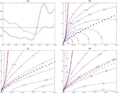
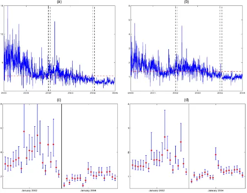
Turning to the properties of the alternative sampling schemes, we note that in the presence of market microstructure noise there is no one sampling scheme that is superior. In fact, whether CTS, BTS, or TTS leads to a lower MSE of the realized variance depends on the specific model parameters and the evo-lution of the intensity process. To illustrate this, we compute the MSE of the realized variance associated with each of the sam-pling schemes across a range of noise ratiosγand sampling fre-quenciesN. The integrated intensity is fixed at(1)=4,000, whereasσε2is set to ensure that=(20%)2annualized. Fur-ther, for the MSE calculations for CTS we consider two dis-tinct intensity paths, one path with little variation beyond the ubiquitous seasonal pattern and the other with large variation [see Fig. 1(a)]. Both intensity paths are rescaled nonparametric smoothing estimates based on IBM data for August 25, 2003 (dashed line) and June 7, 2000 (solid line) and thus represent realistic patterns (for details, see Sec. 6). To facilitate presen-tation, we report the “BTS loss” and “CTS loss,” which are
(a) (b)
(c) (d)
Figure 1. “Inefficiency” of BTS and CTS Across Sampling Frequency and Noise Ratio. (a) The nonparametric smoothing estimates of the trade intensity for IBM on June 7, 2000 ( ) and August 25, 2003 ( ) rescaled to ensure thatΛ(1)=4,000. (b) The isocurves of the BTS loss across a range of sampling frequencies converted to minutes (i.e., 6.5N×60=390N ) on the horizontal axis and the square root of the noise ratio (i.e.,√γ) on the vertical axis. (c) and (d) The corresponding isocurves for the CTS loss using the respective intensity paths of (a). The “+” indicate the optimal sampling frequency for BTS, and while the “◦” indicate the optimal sampling frequency for TTS (b) and CTS [(c) and (d)].
defined as the percentage increase in MSE when moving from TTS to BTS and from BTS to CTS, keeping N fixed. These measures thus represent the cost in terms of MSE associated with the use of a suboptimal sampling scheme.
The results, reported in Figures 1(b)–1(d), can be summa-rized as follows. Consistent with the foregoing discussion, in the absence of market microstructure noise (i.e., γ =0) TTS outperforms BTS and BTS outperforms CTS for any given sam-pling frequency. With noise added to the process, these relation-ships break down, and both the BTS loss and CTS loss can turn negative. This occurs when the sampling frequency and noise ratio combination lies to the left of the solid line. Comparing Figures 1(c) and 1(d) shows that, in line with Proposition 1, the magnitude of the CTS loss is greater when the intensity process is volatile. Additional simulations (not reported here) suggest that an increase in the level of the intensity process causes the solid line to shift leftward, thereby reducing the area in which the CTS and BTS loss is negative. Ultimately, however, these results say little about the performance of the various sampling
schemes in practice unless a sampling frequency is specified. Therefore, to provide the appropriate perspective, we indicate the optimal sampling frequency in the graph, because this is the frequency most relevant for empirical applications. It is clear that in the region around the optimal sampling frequency, TTS outperforms BTS and BTS outperforms CTS, as was the case in the absence of market microstructure noise. Moreover, it is interesting to note that the optimal sampling frequencies for the various schemes lie very close together, suggesting that the sim-ple formula in (15) is more widely applicable to other schemes, at least to a first approximation. All of the foregoing results are robust to alternative choices of model parameters and intensity path specifications.
An issue that remains open at this point is whether (and if so, how) the foregoing results are expected to change when the or-der of the MA process is raised. In particular, what will happen to the MSE and optimal sampling frequency in such a case, and will the properties of the sampling schemes change? To answer the first question, we investigate how the optimal sampling fre-quency and magnitude of the MSE change when moving from
an MA(1) specification to an MA(2). In doing so, we distin-guish among two cases: changeρ2while keeping the variance ofν constant, and change ρ2while keeping the variance ofη constant. The first case corresponds to adding noise, and we find that this leads to an increase in MSE and a decrease of optimal sampling frequency. The second case corresponds to altering the structure of the noise dependence, in which case the results can go either way. Both of these finding are quite intuitive and are robust to the specific choice of parameter values and the order of the MA process. To answer the second question, we redo the foregoing analysis for the MA(2) case, and find that these results are also qualitatively unchanged with higher-order dependence.
4. A SMALL JUMP TO A DIFFUSION?
We now provide an informal discussion of some important differences between the properties of the realized variance de-rived earlier and those obtained in a diffusion setting. First, it is easy to see from (9) that the realized variance is an inconsis-tent estimator of the integrated variance in the current frame-work. For BTS, the variance of the realized variance converges to 3σε2 >0 whenN→ ∞. Intuitively, because the price path follows a pure jump process, there is a point beyond which in-creasing the sampling frequency does not generate any addi-tional information; instead, increasing the sampling frequency will just lead to the addition of more and more 0’s into the sam-pled return series, and hence the inconsistency. This is clearly not the case for a diffusive price process that is of infinite vari-ation and for which realized variance is consistent, at least in the absence of market microstructure noise. Keep in mind that because the sampling frequency for TTS cannot be increased in-definitely (as is possible for BTS or CTS) because it is capped byM(1), the minimum attainable MSE for this scheme is also strictly positive.
Another observation worth highlighting is that for the pure jump process, the bias of the realized variance is bounded when the sampling frequency increases. For instance, for CTS, the maximum attainable bias is equal to
lim
This again contrasts sharply with the results derived for the dif-fusive model, where the bias of the realized variance diverges when the sampling frequency increases (see, e.g., Bandi and Russell 2004a; Zhang et al. 2005). Clearly, the inconsistency of the realized variance and the boundedness of the bias in the cur-rent framework vanishes in the “diffusion limit” as discussed earlier, whereσε2→0, (t)→ ∞ while keeping and σν2
fixed (see Oomen 2005 for more details).
Finally, consider the “rule-of-thumb” optimal sampling fre-quency expression of Bandi and Russell (2004a,b) (see also Aït-Sahalia et al. 2005; Zhang et al. 2005) for continuous semi-martingales,
As pointed out by Bandi and Russell, in practice Nq should
be chosen sufficiently small (i.e., low frequency) forQnot to be severely biased by market microstructure noise, whereas Nα should be set at its maximum possible value. For the CPP–MA(1) model, it is easy to show that for TTS, E[Q] = Nq2σε4(2γ+N−q1(1))2andE[α] ≈σε4(1+2γ )2forNαlarge. Therefore, ignoring any measurement error inαandQ, it fol-lows that
Even though Bandi and Russell derived their optimal sampling frequency in a diffusion setting, the foregoing analysis is still of interest for the simple reason that the CPP in transaction time is equivalent to a Brownian motion that is discretized at regular intervals in calendar time. In this setting, the integrated inten-sity(1)can thus be loosely interpreted as the number of dis-cretization points or observations. In other words, sampling a Brownian motion in calendar time leads to returns that have ex-actly the same properties as those generated by the CPP model in transaction time. Thus, comparing (15) and (16) provides an insight into the “discretization” bias of the optimal sam-pling frequency proposed by Bandi and Russell, which arises in a diffusion setting due to the inevitable lack of an infinite number of transactions in practice. It is clear that there are two sources of bias with opposing effects; that is, 2γNqin the
numerator increases the optimal sampling frequency, whereas the extra term in the denominator decreases the optimal sam-pling frequency. Depending on parameter values, either effect can dominate, although it is likely that in practice the opti-mal sampling frequency is underestimated by the procedure of Bandi and Russell because Nq is small. To illustrate this and
develop some sense for the magnitude of this bias, setγ =2, Nα =(1)=5,000, and Nq=26. The noise ratio and(1)
are in line with estimated values for IBM, whereasNα andNq
are set following the guidelines of Bandi and Russell, that is, Nα as high as possible andNq set to imply a 15-minute
sam-pling frequency (based on a 6.5-hour trading day) for the esti-mation ofQ. With these values,Ntr∗=116 or 3.36 minutes and NBR∗ =101 or 3.86 minutes. Hence there is a discretization bias of about 15%, which goes some way towards explaining the bias in optimal sampling frequency reported in the simulations of Bandi and Russell (2004b). Still, the impact of this bias in terms of MSE is likely to be minimal in practice. For instance, based on (11) and assuming=(20%)2annualized, the cor-responding increase in MSE of the realized variance due to the suboptimal choice of sampling frequency is about 1.5%.
5. SOME EXTENSIONS OF THE CPP–MA MODEL
As discussed earlier, the CPP–MA model in (4) can ac-count for a number of important features of high-frequency data, including serial correlation of returns, stochastic duration and volatility dependence, diurnal patterns in market activity,
and a fat-tailed marginal distribution of returns in calendar time. Nonetheless, the model can be extended to various di-rections, which we briefly outline in this section. For instance, it may be of interest to incorporate a correlation between the efficient price innovation and the market microstructure noise component, that is, E[εjνj] =κσεσν. As argued by Hansen and Lunde (2006), such a noise specification may be appro-priate because it can account for downward-sloping volatility signatures encountered in practice, particularly for mid-quote data (see also Oomen 2006). The present framework can be altered straightforwardly to allow for this, with the only ex-pressions needing changes are those ofq andqin
Appen-dix A. As an illustration, with “correlated” noise it is easy to show that the covariance of returns in calendar time is equal to Eλ[R(ti|τi)R(tj|τj)] = −(κ√γ+γ )σε2e−λi,j(e−λj−1)(e−λi−1), so that when κ <0, the correlation is dampened. To evalu-ate the MSE of the realized variance in this case, one addi-tional parameter must be estimated, which can be done with a moment-matching procedure similar to that outlined later. The only possible complication here is that to identify κ higher-order return moments should be included, which may lead to estimates that can be somewhat erratic or noisy.
Another extension that may be worth pursuing is to re-lax the independence assumption between the trade intensity process λ and the conditional mean and variance of the effi-cient price innovationε. For instance, the market microstruc-ture literamicrostruc-ture (e.g., Admati and Pfeiderer 1988; Easley and O’Hara 1992) makes specific (albeit somewhat contradictory) predictions about the relationship between the trade intensity and return volatility through the level of informed trading. Empirical work by Engle (2000), Ghysels and Jasiak (1998), Grammig and Wellner (2002), and Russell and Engle (2005) has focused on investigating such a relation using extended ver-sions of the seminal autoregressive conditional heteroscedas-ticity model of Engle (1982) and the autoregressive conditional duration (ACD) model of Engle and Russell (1998). The well-documented presence of a leverage effect between the condi-tional mean and volatility of returns (e.g., Black 1976; Heston 1993) further indicates that allowing for correlation between
λandεmay be important. Although these extensions are less straightforward, important progress has been made on this front by Bandi and Russell (2004a) and Barndorff-Nielsen et al. (2006) in a diffusion setting.
Finally, alternative distributions forε(andν) can be consid-ered. A multinomial distribution may be appropriate when price discreteness is a concern (see Griffin and Oomen 2005). Alter-natively, a mixture distribution in the spirit of Kon (1984) can be used to allow for the modeling of skewed, leptokurtic, and multimodal distributions. As an illustration of this, consider the CPP–MA(1) model with constant noise varianceσν2and a mix-ture of two normals for the efficient price innovation, that is,
εj∼
N(0, σ12) with probabilityπ
N(0, σ22) with probability 1−π.
The variance of transaction returns, withh1andh−h1 denot-ing the number of realizations from the first and second mix-ing distribution, is then equal to (h,h1)≡V[r(k|h,h1)] =
hσ22+h1(σ12−σ22)+2σν2forh≥1. With this, it can be shown that
Eλ
exp{iξR(ti|τi)}
∝
∞
h=1
h
h1=0
h!πh1(1−π )h−h1 h1!(h−h1)!
exp
−1
2ξ 2(h,h
1)
λh
i
h!eλi
=(1−exp{−λidec})exp{−ξ2σν2+λi(dec−1)},
wherec= −12ξ2σ22 andd=1−π+πexp{−12ξ2(σ12−σ22)}. Clearly, whenσ12=σ22, it follows thatd=1, so that the char-acteristic function, and hence the moments, correspond to those discussed earlier. Because the covariance of transaction returns is not affected by the mixture distribution, the joint characteris-tic function of calendar time returns can be derived in a similar fashion, albeit with some added notational complexity.
6. MARKET MICROSTRUCTURE NOISE IN
PRACTICE: IBM TRANSACTION DATA
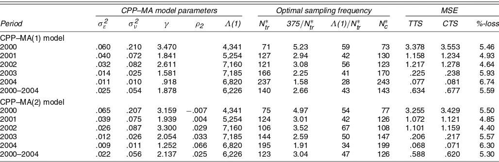
In this section we discuss how the foregoing methodology can be used in practice to determine the optimal sampling fre-quency and measure the efficiency gains and losses associated with alternative sampling schemes. The analysis is based on the CPP–MA(1) and CPP–MA(2) specifications using transaction-level data for IBM. The main findings can be summarized as follows. First, the estimation of the model parameters is straightforward and delivers sensible results, whereas simula-tion results indicate that the inevitable measurement error in estimated parameters does not significantly bias the model-implied optimal sampling frequency and MSE. Second, the em-pirical results for the CPP–MA(1) and CPP–MA(2) models are very similar, suggesting that for IBM over the sample period considered here, there is no need to include higher-order de-pendence in the noise component. Third, the optimal sampling frequency for the IBM transaction data varies significantly over time but declines steadily from about 5 minutes in 2000 to 1.5 minutes in 2004. Fourth, sampling regularly spaced in trans-action time outperforms the common practice of sampling in calendar time for each day in the sample, with the greatest MSE reductions on days with irregular trading patterns.
6.1 Estimation of the Model Parameters
The empirical analysis concentrates on the CPP–MA(2) model as specified by (4). The relevant moment expressions are given in Appendix B. For simplicity, we assume thatµε=0. The remaining model parameters {σε2, σν2, ρ2}and the inten-sity processλ(t)together with(1)are estimated for each day in the dataset separately using all available transaction prices and transaction times. In particular, the model parameters are estimated using a simple method-of-moments procedure that matches the sample variance and autocovariances of transac-tion returns for a given day to their theoretical counterparts, that is,
Er(k|1)r(k−1|1)= −σν2(1−ρ2)2,
Er(k|1)r(k−2|1)= −ρ2σν2,
and
E[r(k|1)2] =σε2+2σν2(ρ22−ρ2+1),
whereσν2>0 and|ρ2|<1. Similarly,(1)can be estimated unbiasedly as the number of transactions, that is,Eλ[M(1)] =
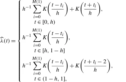
(1). Daily estimates of {λ(t),t ∈ [0,1]} are obtained us-ing a standard nonparametric smoothus-ing estimator (Diggle and Marron 1988) taking the form
λ(t)= (converted to the unit interval) for a particular day, h is the bandwidth, andK(x) is a kernel with support on the interval x∈ [−1,1]. It is clear from (17) thatλ(t)is obtained by lo-cally averaging the number of transactions over the interval
[t−h,t+h] using a kernel. Because estimates of λ(t) close to the edges (i.e., t∈ [0,h) and t ∈(1−h,1]) will be bi-ased downward due to the absence of transactions outside the unit time interval, a “mirror image adjustment” of Diggle and Marron (1988) is used to counter this effect; that is, the first and third lines in (17) constitute the adjustment. Implementa-tion of the estimator in (17) requires a specific choice of kernel and bandwidth. It is well known from the literature on non-parametric estimation that the choice of bandwidth is crucial because it balances the trade-off between reducing the variance of the estimator by increasingh, thereby extending the smooth-ing horizon and reducsmooth-ing the bias of the estimator by decreassmooth-ing h. The choice of kernel, on the other hand, is of secondary im-portance. Therefore, in this article we simply follow Diggle and Marron (1988) and use a quartic kernel,K(x)=.9375(1−x2)2
forx∈ [−1,1]and 0 otherwise.
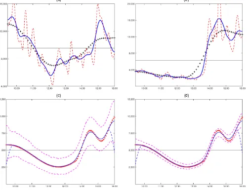
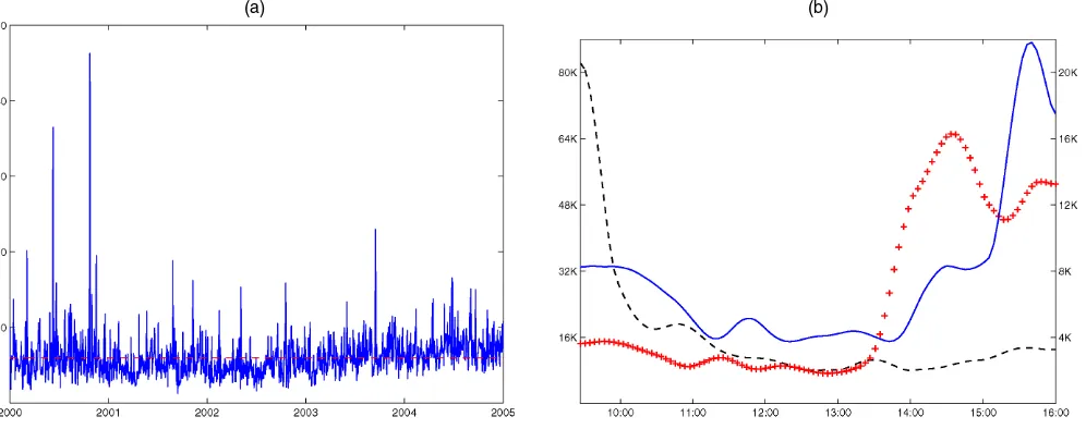
To guide the choice of bandwidth, we experiment exten-sively with actual IBM transaction data. As an illustration, Fig-ures 2(a) and 2(b) plot the intensity estimates for various values ofhusing data on two distinct days: November 14, 2002, with a familiar U-shaped intensity pattern, and June 7, 2000, with a highly irregular evolution of the intensity process. Although the intensity process is inherently unobservable, by eyeballing the graphs, it seems reasonable to conclude that the solid line cap-tures the salient feacap-tures of the process. The associated band-width ofh=.075 corresponds roughly to a smoothing window of 1/2 hour backward and forwards (i.e.,.075×375 minutes). Substantially reducing the bandwidth can lead to an excessively volatile estimate of the intensity process, as illustrated by the dashed line with h=.025. Increasing the bandwidth, on the other hand, may cause the estimate to miss some important local variation of the intensity process, as is illustrated by the cross-dotted line withh=.225. Because these results are rep-resentative for the dataset as a whole and are robust to different
intensity patterns, we decide to use a bandwidth of h=.075 throughout. Given the high level of transaction intensity for IBM (an average of more than 6,000 trades per day), it may be argued that this choice of bandwidth is on the conservative side and possibly could be lowered, especially on busy days. It is worth pointing out, however, that oversmoothing only leads to understating the virtues of transaction time sampling, because the MSE for CTS generally increases with increasing variability of the intensity process.
In addition to the choice of bandwidth, it is important to gauge the accuracy of the intensity estimates and the effec-tiveness of the mirror-image bias correction around the edges. To address both issues, we use simulations. In particular, we fix an intensity path {λ(t),t∈ [0,1]} and use this to simu-late K sets of transaction times, that is, {t0(i),t(1i), . . . ,t(Mi)
i}for i=1,2, . . . ,K and Eλ[Mi] =(1). Based on this, we then
use (17) to obtain K corresponding estimates of the inten-sity path, that is, {λ(i)(t),t∈ [0,1],i=1,2, . . . ,K}. Because a volatile low-intensity path is most difficult to estimate, we specify the intensity process as λ(t)∝2+.2πt+cos(2πt)− .75(cos(4(2πt−4))−1)1t≥2/π, which captures a linear trend (i.e., seasonal pattern) as well as some irregularities and distin-guish among two cases, (1)=500 and (1)=5,000. Fur-ther, we set h=.075 andK=1,000. Figures 2 (c) and 2(d) report the intensity path (cross-dotted line) together with the mean (solid line) and the first and 99th pointwise percentiles (dashed lines) of the bias-corrected intensity estimates. The downward-sloping dashed lines around the edges represent the intensity estimates when no bias correction is applied. From these results, it is clear that the nonparametric smoothing esti-mator delivers accurate and virtually unbiased estimates of the intensity process. Even when the integrated intensity is set to 500, the confidence bounds indicate that the estimator picks up the variation of the intensity path. Increasing(1)to 5,000 re-sults in highly accurate estimates. Moreover, the mirror-image adjustment around the edges is clearly very effective in reduc-ing the bias.
Finally, before turning to empirical analysis, we conduct some further simulations to gauge the impact of measurement error in the model parameters and the intensity process on the estimates of the optimal sampling frequency and MSE loss. In particular, we use the CPP–MA(1) model withγ =2 to simu-late transaction prices and transaction times. The intensity pat-tern is set equal to that of the IBM intensity estimate of June 7, 2000 [i.e., the solid line in Fig. 1(b)] and then rescaled to distin-guish among two cases, an “illiquid” market with(1)=500 and a “liquid” market with(1)=5,000, keeping=(20%)2
by varying σε2 accordingly. Based on the simulated data, we then use moment-matching and nonparametric smoothing (with h=.075) as described earlier to obtain estimates of the model parameters and the intensity process. With these estimates, we compute the model-implied optimal sampling frequencies for TTS, BTS, and CTS together with the BTS and CTS losses. Table 1 reports the results based on 10,000 simulation repli-cations. Regarding the model parameters, the simulations in-dicate that the moment-matching procedure delivers unbiased estimates of σε2 andσν2. Increasing the level of the intensity process leads, as expected, to higher accuracy. The estimated noise ratio, obtained as the ratio of estimates ofσν2andσε2, is
(a) (b)
(c) (d)
Figure 2. Nonparametric Estimation of the Trade Intensity Process. (a) and (b) The nonparametric smoothing estimates of the trade intensity for IBM on November 14, 2002 and June 7, 2000. The bandwidth is set equal to h=.025≈10 minutes ( ), h=.075≈30 minutes ( ), and h=.225≈1.5 hours (+++). (c) and (d) The nonparametric smoothing estimates ( ) plus 1% and 99% bootstrapped confidence bounds ( ) for givenλ(t) (+++) withΛ(1)=500 andΛ(1)=5,000. The intensity specification isλ(t)∝2+.2πt+cos(2πt) −.75(cos(4(2πt−4))−1)1t≥2/π
for t∈[0, 1]. The downward sloping dashed lines at the edges represent the intensity estimates when no bias correction is used.
Table 1. Simulation Results
CPP–MA(1) model parameters Optimal sampling frequency
σε2 σν2 γ Ntr∗ Nb∗ Nc∗
BTS loss %
CTS loss %
“Illiquid” market:(1)=500
True .3175 .6349 2.0000 25.00 25.00 29.00 3.830 26.95 Mean .3169 .6357 3.3169 24.77 24.77 29.07 3.910 26.77 Median .3170 .6329 1.9892 24.61 25.00 29.00 3.850 26.44 SD .1041 .0855 8.6457 7.570 7.570 9.270 1.320 7.670 5th percentile .1455 .5003 1.0658 12.72 13.00 15.00 1.900 21.90 95th percentile .4887 .7799 5.1359 37.49 37.50 45.00 6.130 31.01 “Liquid” market:(1)=5,000
True .0317 .0635 2.0000 116.0 116.0 135.0 2.050 32.54 Mean .0318 .0635 2.0289 115.7 115.7 134.9 2.050 31.27 Median .0318 .0634 1.9978 115.5 115.0 135.0 2.050 31.26 SD .0033 .0028 .2963 10.97 10.98 12.83 .210 1.030 5th percentile .0263 .0590 1.6051 97.81 98.00 114.0 1.720 29.60 95th percentile .0372 .0681 2.5634 133.7 134.0 156.0 2.400 32.98
NOTE: This table reports the median CPP–MA(1) parameter estimates (σ2
ε×1e6,σν2×1e6), plus associated optimal sampling frequency statistics, based on simulated data using 10,000
replications.