Power Quality Analysis Using Frequency Domain
Smooth-Windowed Wigner-Ville Distribution
Abdul Rahim Abdullah
1, Nurul Ain Mohd Said
2, Ahmad Zuri Sha’ameri
3, Fara Ashikin Ali
4 1, 2, 4Faculty of Electrical Engineering , Universiti Teknikal Malaysia Melaka, 76100 Malacca, Malaysia
3
Faculty of Electrical Engineering , Universiti Teknologi Malaysia 81310 Johor, Malaysia
1
Abstract — Power quality has become a great concern to all electricity consumers. Poor power quality can cause equipment failure, data and economical losses. An automated monitoring system is needed to ensure signal quality, reduce diagnostic time and rectify failures. This paper presents the analysis of power quality signals using frequency domain smooth-windowed Wigner-Ville distribution (FDSWWVD). The power quality signals focused are swell, sag, interruption, harmonic, interharmonic and transient based on IEEE Std. 1159-2009. The TFD represents signal jointly in time-frequency representation (TFR) with good frequency and time resolution. Thus, it is very appropriate to analyze the signals that consist of multi-frequency components and magnitude variations. However, there is no fixed kernel of the TFD can be used to remove cross-terms for all types of signals. A set of performance measures is defined and used to compare the TFRs to identify and verify the TFD that operated at optimal kernel parameters. The result shows that FDSWWVD offers good performance of TFR and appropriate for power quality analysis.
I. INTRODUCTION
Power quality has become a great concern to all electricity consumers.Sensitive equipment and non-linear loads are now more common place in both industrial sectors and domestic environment [1]. Low power quality signals can cause many serious problems to the equipment such as short lifetime, malfunctions, instabilities and interruption. Thus, there is a need for heightened awareness of power quality among electricity users. Specifically, industries which are requiring ultra-high availability of service and precision manufacturing systems are very sensitive to power quality problems [2]. The utilities or other electric power providers have to ensure a high quality of their service to remain competitive and to retain the customers.
The power quality term was earliest mentioned in a study published in 1968 [3] and many techniques were presented by various researchers for power quality signals analysis [4]. The most widely used is Fourier analysis but it does not suitable for non-stationary signals [5]. This is due to the technique provides information only about the existence of a certain frequency component but does not give information about component appearance time. To solve the problem, short-time
Fourier transform (STFT) [6] from linear time-frequency distribution (TFD) was introduced. This technique provides temporal and spectral information of a signal by representing it jointly in time-frequency representation (TFR). However, STFT still has limitation of a fixed window width. The trade-off between the frequency resolution and time resolution should be determined to observe a particular characteristic of the signals.
As an alternative to resolve the fixed resolution problem of STFT, wavelet transform (WT) which is another linear TFD was proposed [7]. WT offers high time resolution for high frequency component and high frequency resolution for low frequency component [8]. Thus, the technique is suitable to detect the duration of high frequency signal such as transient. However, for low frequency signals, typically sag, swell and interruption, it does not produce reliable results [9]. In addition, WT also exhibits some disadvantages such as its computation burden, sensitivity to noise level and the dependency of its accuracy on the chosen basis wavelet [10] [11].
Bilinear TFD is known as better distribution than linear TFD because it provides good resolution in both time and frequency domain [12]. However, it suffers from the presence of cross-terms that can result in misinterpretation of the true signal characteristics. Besides, there is no fixed kernel that can be used to remove the cross-terms for all types of signals [13]. Thus, the optimal kernel parameter of the signal needs to be identified for implementing the TFD.
reduced by using larger windows for time smoothing but it also causes reduction in the time resolution. The implementation of SWWVD in frequency domain may overcome the SWWVD limitations and reduce computation time.
This paper presents the implementation of bilinear TFD which is frequency domain smooth-windowed Wigner-Ville distribution (FDSWWVD) for power quality signals analysis. This TFD consists of a separable kernel which its parameters are estimated from the Doppler-frequency signal characteristics. From the appropriate choice of the kernel parameters, the auto-terms are preserved and the cross-terms are removed. A set of performance measures is defined based on the main-lobe width (MLW), peak-to-side lobe ratio (PSLR), signal-to-cross-terms ratio (SCR) and absolute percentage error (APE) to quantify the accuracy of the resulting TFR.
II. SIGNAL MODEL
This paper divides the power quality signals into three classes: voltage variation for swell, sag and interruption signal, waveform distortion for harmonic and interharmonic, and transient signal. The signal models are formed as a complex exponential signal based on IEEE Std. 1159-2009 and can be defined as
∑
=−
− Π =
3 1
1 2
) ( )
( 1
k
k k k t f j
vv t e A t t
x π (1)
t f j t f j
wd t e Ae
x ()= 2π0 + 2π1 (2)
) (
) ( )
(
1 2 ) ( 2 ) /( ) ( 25 . 1
3 1
1 2
1 2 1 2 1 1
t t e
Ae
t t e
t x
t t f j t t t t k
k k t f j trans
− Π +
− Π =
− −
− −
=
−
∑
π π
(3)
⎩ ⎨
⎧ ≤ ≤ −
=
Π −
elsewhere
0
0 for 1 )
( k k 1
k
t t t
t (4)
where k is the signal component sequence, Ak is the signal
component amplitude, f1 and f2 are signal frequency, t is the
time and Π(t) is a box function of the signal. In this analysis, the parameters are set similar to [14] for comparison purpose.
III. FREQUENCY DOMAIN SMOOTH-WINDOWED WIGNER
-VILLE DISTRIBUTIONS
Smooth-windowed Wigner-Ville distribution (SWWVD) has a separable kernel [15] where it can reduce the effects of the interferences or cross-terms and at the same time, having a high time-frequency resolution. The TFD can be expressed as
∫
∞
∞ −
−
= H t K tτ wτ πfτ dτ
f t
P x
t x
SWWVD (, ) ()* (, ) ( )exp( 2 ) )
(
, (5)
where H(t) is the time smooth (TS) function, w(τ) is the lag
window function and kx(υ,f) is the bilinear product of the
signal of interest, x(t). In this paper, Hamming window is used as the lag window while raised-cosine pulse as the TS function [16]. They are, respectively, defined as
⎪⎩ ⎪ ⎨
⎧ + − ≤ ≤
=
elsewhere
0
cos 64 . 0 54 . 0 )
( g g g
T T
T w
τ πτ
τ (6)
⎩ ⎨
⎧ + ≤ ≤
=
elsewhere
0
0 ) / cos( 1 )
(t t Tsm t Tsm
H π (7)
The bilinear product can be represented in frequency domain [17] and the corresponding definition is
τ
υ
τ
π
τ
τ
υ
dtd t f j
t x t
x f
kx
)) (
2 exp(
) 2 / ( ) 2 / ( ) ,
( *
+ −
− +
=
∫∫
(8)
If m and n are defined as
2 /
; 2
/ τ
τ = − +
=t n t
m (9)
then using the Jacobian yields
dmdn
dtdτ = (10)
With these substitutions, equation (8) can be factored into
) 2 / ( ) 2 / (
) ] 2 / [ 2 exp( ) (
) ] 2 / [ 2 exp( ) ( ) , (
* *
υ
υ
υ
π
υ
π
υ
− +
=
− + −
=
∫
∫
∞
∞ − ∞
∞ −
f X f
X
dn n f
j n z
dm m f
j m x f
kx
(11)
Noting that the kx(υ,f) has similar form to Kx(t,τ) in the
Doppler-frequency domain. By using the properties of the Fourier transform for convolution and product between two signals, the SWWVD in equation (5) can be defined in frequency domain as
∫
∞
∞ −
−
= W f K υ f hυ πυt dυ
f t
P x
f x
SWWVD (, ) ( ) * ( , ) ( )exp( 2 ) )
(
, (12)
where W(f) is the lag window in frequency domain, h(υ)is the
TS function in Doppler domain and the asterisk with f denotes the frequency-convolution of the signals.
)
REPRESENTATION
The bilinear product of a signal in Doppler-frequency representation is divided into two components which are auto-terms and cross-auto-terms. It can be defined as
)
The auto-terms are normally located at frequency axis (υ =
0) while the cross-terms can be anywhere. Thus, TS function is used to remove the cross-terms which are located away from the frequency axis and lag window is for the cross-terms that have lag-frequency component.
A. Bilinear Product of Voltage Variation Signal
In frequency domain analysis, the signal in equation (1) is transformed to frequency domain by using Fourier transform and its frequency domain representation is defined as
Since auto-terms are the bilinear product of the same signal components while cross-terms are the bilinear product of the different signal components, they can be defined, respectively, as
)
Based on equation (17) and (18), the auto-terms have no frequency component while the cross-terms have lag-frequency component at f = f0. Both terms are centred at f = f0
and υ = 0 as shown in Fig. 1.
Fig. 1: Bilinear product of the voltage variation in Doppler-frequency representation
By using the convolution properties [18], the convolution between the lag window and cross-terms can be defined as
dk
f0
From the equations above, lag window parameter, Tg, should be set less than or equal to the smallest value between (t2 - t1)/2, (t3 - t1)/2 and (t3 - t2)/2 to remove the cross terms. In
However, similar to the analysis in time domain [20], lag window should cover at least one cycle of fundamental signal such that Tg≥ 1/2f0.
B. Bilinear Product of Waveform Distortion Signal
Waveform distortion signal in equation (2) consists of two frequency components and its frequency domain representation is expressed as
)
The auto-terms and cross-terms of the signal can be defined, respectively, as
)
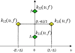
The equations above indicates that there are two auto-terms which are located at the frequency axis and centred at f
= f0 and f1, respectively, as shown in Fig. 2. Besides that, two
cross-terms are located away from the frequency axis which are at f = (f1 + f0)/2, υ = (f1 – f0) and f = (f1 + f0)/2, υ = - (f1 – f0)
and have no frequency component.
Fig. 2: Bilinear product of the waveform distortion signal in frequency-Doppler representation
In Doppler-frequency representation, the TS function behaves like a window similar to lag window in time-lag domain. This is due to it can remove the cross-terms which are located away from the frequency and preserves the auto-terms at the origin of the Doppler axis. Since the cross-terms are located at |υ|= (f1 – f0), the Doppler cut-off frequency of the
TS function should be set such that υc ≤ | f1 – f0|. It can be
achieved by setting the TS function parameter as
0
The lag window is also applied to this signal to set the desirable lag-frequency resolution, Δf, of the TFR [20]. Thus,
Tg should be set greater than or equal to 1/2Δf to set the lag frequency resolution such that Δf ≤ f1/2 to differentiate
harmonic and interharmonic frequency components.
C. Bilinear Product of Transient Signal
Transient signal as in equation (3) can defined in frequency domain as
)
while another signal component has frequency component at f
= f0. Its auto-terms and cross-terms can be, respectively,
defined as
) kcross
υ
In equation (32), three auto-terms are located at the frequency axis. An auto-term is centered at f = f0 while the
Fig. 3. There are six cross-terms where two cross-terms are located at f = (f1T + f0)/2, υ = (f1T – f0), two cross-terms are at f
= (f1T + f0)/2, υ = - (f1T – f0) and another are at f = f1T, υ = 0 as
expressed in equation (33). Thus, four cross-terms are located away from the frequency axis while two cross-terms share the same location with the auto-terms at the frequency axis and at f = f1T.
Fig. 3: Bilinear product of the transient signal in Doppler- frequency representation
The four cross-terms are located away from the frequency axis which is at υ= | f1T – f0|. Thus, the TS function is
implemented similar to the waveform distortion signal to remove the cross-terms. To simply the calculation, since f1T≈ f1, the Doppler cut-off frequency is set at υc ≤ | f1 – f0| by
setting Tsm such that
0 1 2
3 f f Tsm
−
≥ (39)
For the cross-terms that are located at the frequency axis, lag window is employed since the cross-terms have lag-frequency component. This application is similar to the voltage variation signal and same observation can be made. Based on the Eigen function properties, the output for convolution between lag window and these cross-terms can be defined as
⎥ ⎥ ⎥ ⎥ ⎥
⎦ ⎤
⎢ ⎢ ⎢ ⎢ ⎢
⎣ ⎡
+ − =
− = −
− −
− − = −
− + −
2 / ) ( ) )( 2 ( 2
2 / ) ( )
)( 2 ( 2
1 , 1 2
, 1 sinc 2 / ) ( 2 1 2 )
21 , 12 (
1 2 1
1 2
1 2 1
1 2
1 2
) (
) (
) ,
( )
, (
t t f
f t t π j
t t f
f t t π j
T T t
t v j cross
w e
w e
f f k
e t t A f r
T T
τ τ π
τ τ
υ υ
(40)
In order to remove the cross-terms, w(τ) which is at |τ|= (t2
- t1)/2 should be set at zero. Thus, the lag window parameter is
set such that Tg≤ (t2 - t1)/2. However, an appropriate setting
for Tg and Tsmshould be chosen in order to remove the
cross-terms, preserve the auto-cross-terms, set desirable frequency resolution as well as reduce computation complexity and memory size of the TFR.
V. RESULT
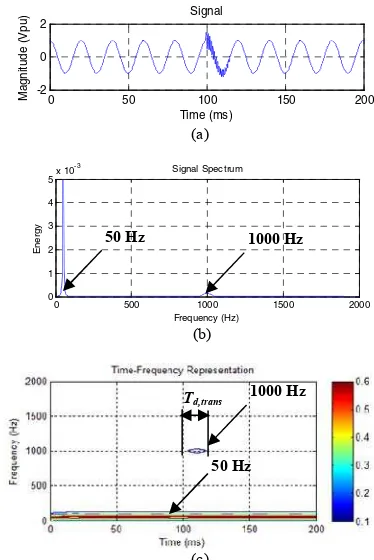
Transient signal in time domain, frequency domain and its TFR are shown in Fig. 4. Fig. 4(a) presents the magnitude of the signal increases at 100 ms and its duration is 15 ms. For Fig. 4(b), the signal spectrum shows two frequency components which are at 50 and 1000 Hz while the others are zeros. Its TFR as shown in Fig. 4(c) demonstrates that transient occurs at 1000 Hz between 100 and 116 ms. This example shows that the two frequency components need to be considered for calculating FDSWWVD. As a result, it reduces the computation complexity.
(a)
(b)
(c)
Fig. 4: a) Interruption signal in time domain and b) frequency domain and c) its TFR
The performance of FDSWWVD with various kernel parameters is also verified in terms of MLW, PSLR, SCR and APE for power quality signals as discussed in [20]. By using similar parameters as in [14], the performance of SWWVD and FDSWWVD is compared as presented in Table 1.
It can be seen that, for every signal, FDSWWVD gives small different results compared to SWWVD. This is due to small sample value of the signal in frequency domain are not considered to reduce computation complexity for calculating FDSWWVD and the same time also offers good TFR. Thus, the FDSWWVD is suitable to be implemented to power quality signals detections and classification purpose.
0 50 100 150 200 -2
0 2
Signal
Time (ms)
M
a
gn
it
ud
e (V
p
u
)
0 500 1000 1500 2000
0 1 2 3 4 5x 10
-3 Signal Spectrum
E
n
er
gy
Frequency (Hz)
50 Hz 1000 Hz
0 υ
F0 F1T
(f1T+ f0)/2
-(f1T –f0) (f1T –f0)
f
k33(υ, f )
K31(υ, f )+ k32(υ, f ) K11(υ, f )+ k22(υ, f )+ k12(υ, f )+ k21(υ, f )
k13(υ, f )+ k23(υ, f )
Td,trans 1000 Hz
TABLE I
PERFORMANCE COMPARISON BETWEEN SWWVD AND FDSWWVD AT THE
OPTIMAL KERNEL
Signal Performance
Measures SWWVD FDSWWVD
V
o
lt
ag
e V
ar
ia
ti
on
S
ign
al
Swell
MLW (Hz) PSLR (dB) SCR (dB)
APE (%)
25 614.815 15.6408 0.20833
25 256.39 16.572 0.2083
Sag
MLW (Hz) PSLR (dB) SCR (dB)
APE (%)
25 614.815 17.7996 0.625
25 129.3 18.610 0.4166
Interruption
MLW (Hz) PSLR (dB) SCR (dB)
APE (%)
25 614.815 55.4463 0.625
25 87.358 14.100 4.375 Kernel
parameters
Tg(ms)
Tsm(ms)
10 0
10 0
W
ave
fo
rm
D
is
to
rt
ion
S
ign
al
Harmonic
MLW (Hz) PSLR (dB) SCR (dB)
APE (%)
6.25 664.295 41.7393 0.125
12.5 48.456 12.278 0.0700 Kernel
parameters
Tg(ms)
Tsm(ms)
20 7.5
20 7.5
Interharmonic
MLW (Hz) PSLR (dB) SCR (dB)
APE (%)
6.25 655.776
42.256 0.125
12.5 47.315 12.267 0.3454 Kernel
parameters
Tg(ms)
Tsm(ms)
20 6.67
20 6.67
T
ra
n
si
en
t
S
ign
al Transient
MLW (Hz) PSLR (dB) SCR (dB)
APE (%)
25 86.1447 14.1705 1.66667
25 93.2472
15.582 0.555556 Kernel
parameters
Tg(ms)
Tsm(ms)
10 1.578
10 1.578
VI.CONCLUSION
FDSWWVD presents power quality signals in time-frequency representation with good time and time-frequency resolution. However, each type of the signals requires different kernel parameters of the TFD to obtain the optimal TFR. Thus, a set of performance measures which are MLW, APE, SCR and PSLR is used to identify and verify the optimal kernel. The results show that FDSWWVD offers good performance of the TFR and give the optimal kernel similar to SWWVD. In addition, the TFD is implemented in Doppler-frequency domain that reduces computation complexity compared to SWWVD which is performed in time-lag representation.
ACKNOWLEDGEMENT
The authors would like to thank to Universiti Teknikal Malaysia Melaka (UTeM) for financial support and providing the resources for this research.
REFERENCES
[1] Y. Krisda, P. Suttichai and O. Kasal, “A Power Quality Monitoring
System for Real-Time Fault Detection”, IEEE International
Symposium on Industrial Electronics (ISIE 2009), pp. 1846-1851, July 2009.
[2] B. R. Godoy, O. P. J. Pinto and L. Galotto, “Multiple Signal Processing Techniques Based on Power Quality Disturbance Detection, Classification, and Diagnostic Software”, International Conference on Electrical Power Quality and Utilisation, pp. 1-6, Oct. 2007.
[3] W. G. Morsi and M. E. El-Hawary, "Fuzzy-Wavelet-Based Electric Power Quality Assessment of Distribution Systems Under Stationary
and Nonstationary Disturbances”, IEEE Transactions on Power
Delivery, vol. 24, no. 4, pp. 2099-2106, 2009.
[4] D. Saxena, K. S. Verma and S. N. Singh, “Power Quality Event
Classification: An Overview and Key Issues”, International Journal of Engineering, Science and Technology, Vol. 2, No. 2, pp. 186-199, 2010.
[5] J. J. Tomic, M. D. Kusljevic and D. P. Marcetic, “An Adaptive Resonator-Based Method for Power Measurements According to the
IEEE Trial-Use Standard 1459-2000”, IEEE Transactions on
Instrumentation and Measurement, vol. 2, no. 2, pp. 250-258, 2010.
[6] A.R. Abdullah, N.M. Saad, A.Z. Sha’ameri, “Power Quality
Monitoring System Utilizing Periodogram and Spectrogram Analysis
Techniques”, IEEE International Conference on Control,
Instrumentation and Mechatronics Engineering., pp. 770-774, 2007. [7] J. Breckling, The Analysis of Directional Time Series: Applications to
Wind Speed and Direction, ser. Lecture Notes in Statistics. Berlin, Germany: Springer, 1989, vol. 61.
[8] Z. Shi, L. Ruirui, Q. Wang, J. T. Heptol and G. Yang, “The Research of Power Quality Analysis Based on Improved S-Transform”, International Conference on Electronic Measurement & Instruments (ICEMI '09),pp. 477-481, 2009.
[9] A. Andreotti, A. Bracale, P. Caramia and G. Carpinelli, “Adaptive Prony Method for the Calculation of Power Quality Indices in the
Presence of Nonstationary Disturbance Waveforms”, IEEE
Transactions on Power Delivery, vol. 24, no. 2, pp. 874-883, 2009. [10] T. Radil, P. M. Ramos and A. C. Serra, “Detection and Extraction of
Harmonic and Non-Harmonic Power Quality Disturbances using Sine Fitting Methods”, International Conference on Harmonics and Quality of Power (ICHQP 2008),pp. 1-6, 2008.
[11] F. Zhao and R. Yang, “Power-Quality Disturbance Recognition Using S-Transform”, IEEE Transactions on Power Delivery, Vol. 22, pp. 944-950, April 2007.
[12] A. M. Youssef, T. K. Abdel-Galil, E. F. El-Saadany and M. M. A. Salama, “Disturbance Classification Utilizing Dynamic Time Warping Classifier,” IEEE Transactions on Power Delivery, vol. 19, no. 1, pp. 272–278, Jan. 2004.
[13] P. J. Schreier, “A New Interpretation of Bilinear Time-Frequency Distributions”, IEEE International Conference on Acoustics, Speech and Signal Processing, pp. 1133-1136, April 2007.
[14] A. R. Abdullah and A. Z. Sha’ameri, “Power Quality Analysis using
Smooth-Windowed Wigner-Ville Distribution”, International
Conference on Information Science, Signal Processing and their Applications (ISSPA 2010), pp. 798-801, 2010.
[15] D. Boutana, B. Barkat and F. Marir, “A proposed High-Resolution Time-Frequency Distribution for the Analysis of Multicomponent and Speech Signals”, International Conference on Science, Engineering and Technology, vol. 2, Jan. 2005.
[16] T. J. Lynn and A. Z. Sha’ameri, “Adaptive Optimal Kernel Smooth-Windowed Wigner-Ville Distribution for Digital Communication Signal”, EURASIP Journal on Advances in Signal Processing, 2008. [17] B. Boashash, Time-Frequency Signal Analysis and Processing: A
comprehensive Reference, Amsterdam: Elsevier, 2003.
[18] H. J. Bollen and Y. H. Gu, Signal Processing of Power Quality Disturbances, Wiley-Interscience, 2006.
[19] H. Ishibuchi, Y. Kaisho, Y. Nojima, “Designing Fuzzy Rule-Based Classifiers That Can Visually Explain Their Classification Results to Human Users”, International Workshop on Genetic and Evolving Systems (GEFS 2008), pp. 5-10, 2008.