Conference paper

MULTISENSOR MULTITEMPORAL DATA FUSION

USING THE WAVELET TRANSFORM

Sherin Ghannam1, Mahmoud Awadallah1, A. Lynn Abbott1 and Randolph H. Wynne2

1

Bradley Department of Electrical and Computer Engineering 2

Department of Forest Resources and Environmental Conservation Virginia Tech, Blacksburg, Virginia, USA

{sghannam,mawadala,abbott,wynne}@vt.edu

Commission VI, WG VI/4

KEY WORDS: Fusion, multiresolution, multitemporal, wavelet

ABSTRACT:

Interest in data fusion, for remote-sensing applications, continues to grow due to the increasing importance of obtaining data in high resolution both spatially and temporally. Applications that will benefit from data fusion include ecosystem disturbance and recovery assessment, ecological forecasting, and others. This paper introduces a novel spatiotemporal fusion approach, the wavelet-based Spatiotemporal Adaptive Data Fusion Model (WSAD-FM). This new technique is motivated by the popular STARFM tool, which utilizes lower-resolution MODIS imagery to supplement Landsat scenes using a linear model. The novelty of WSAD-FM is two-fold. First, unlike STARFM, this technique does not predict an entire new image in one linear step, but instead decomposes input images into separate “approximation” and “detail” parts. The different portions are fed into a prediction model that limits the effects of linear interpolation among images. Low-spatial-frequency components are predicted by a weighted mixture of MODIS images and low-spatial-frequency components of Landsat images that are neighbors in the temporal domain. Meanwhile, high-spatial-frequency components are predicted by a weighted average of high-spatial-high-spatial-frequency components of Landsat images alone. The second novelty is that the method has demonstrated good performance using only one input Landsat image and a pair of MODIS images. The technique has been tested using several Landsat and MODIS images for a study area from Central North Carolina (WRS-2 path/row 16/35 in Landsat and H/V11/5 in MODIS), acquired in 2001. NDVI images that were calculated from the study area were used as input to the algorithm. The technique was tested experimentally by predicting existing Landsat images, and we obtained R2 values in the range 0.70 to 0.92 for estimated Landsat images in the red band, and 0.62 to 0.89 for estimated NDVI images.

1. INTRODUCTION

Data fusion is the process of merging or combining data from several sources. For certain applications, data fusion makes it possible to obtain results of better quality and/or quantity than is feasible from a single data source alone. In the field of remote sensing, for instance, data fusion may involve images that are obtained from different sensing platforms, or possibly from different spectral bands of a single sensor. An example of this is merging a high-resolution panchromatic image with a low-resolution multispectral image of the same scene, to obtain a high-resolution multispectral image. Another well-known example involves the merging of images from satellites with high-resolution images from airborne platforms. Data fusion may also involve substantially different sensing modalities, such multispectral imagery with radar, lidar, or digital elevation maps (Campbell and Wynne, 2011; Shi et al., 2003).

Spaceborne sensing of the earth’s surface presents particular challenges that can benefit from data fusion. The problem of interest here involves satellite-based tracking of change over time, for a given land region. Through such monitoring it is possible perform tasks as crop-growth assessment and detection of intraseasonal ecosystem disturbances. The ability to detect change over time, however, depends directly on the temporal resolution of the imagery that can be acquired. Temporal resolution, in turn, depends on the length of time that is required for a satellite to complete one entire orbit cycle. For example, the revisit period for Landsat 7 is 16 days, and cloud cover or

other weather-related phenomena can reduce the temporal resolution further.

This paper is concerned with the problem of combining imagery from different satellites, obtained at different times, in order to improve the effective spatiotemporal resolution for a given part

of the earth’s surface. This goal is possible by fusing imagery from a high-resolution platform such as Landsat, with imagery that is lower in spatial resolution but higher in temporal resolution. This fusion of data makes it feasible to detect changes over shorter time intervals than is possible with Landsat monitoring alone.

Numerous image fusion algorithms have been proposed to increase the temporal frequency of moderate spatial resolution data (Gao et al., 2006; Hilker et al., 2009a; Hilker et al., 2009b; Zhang et al., 2013). One of the most widely used algorithms is the Spatial and Temporal Adaptive Reflectance Fusion Model, or STARFM (Gao et al., 2006). This approach utilizes Moderate-resolution Imaging Spectroradiometer (MODIS) imagery to supplement the Landsat scenes. MODIS has a revisit period of 1 day, but is much lower in spatial resolution than Landsat. STARFM estimates the predicted surface reflectance by a weighted sum of the spectrally similar neighborhood information from both Landsat and MODIS reflectance at other observed dates. This approach has proved to be effective for many applications, including monitoring of seasonal changes in vegetation cover (Gao et al., 2006; Hilker et al., 2009b) and for monitoring large changes in land use (Hansen et al., 2008;

Potapov et al., 2008). The model was even modified to accommodate thermal infrared images for prediction of land surface temperatures (Weng et al., 2014).

To deal with the problem of heterogeneous (“mixed”) pixels, Zhu et al. (2010) developed an enhanced STARFM (ESTARFM) approach by introducing a conversion coefficient into the fusion model. This addition represents the ratio of change between the MODIS pixels and spectral ETM+ end-members, which are the “pure” spectra corresponding to each of the land cover classes. The enhanced approach provides a solution for the heterogeneous pixels, but it still cannot accurately predict short-term transient changes that have not been captured in any of the observed fine-resolution images.

Another data fusion system is Spatial Temporal Adaptive Algorithm for mapping Reflectance Change (STAARCH) (Hilker et al., 2009a), which was developed to address a different limitation of STARFM. This system tracks disturbance events using Tasseled Cap Transformations of both Landsat and MODIS reflectance data.

Images could also be treated in a 1D fashion by tracking the changes from date to date for each pixel. An approach based on Fourier regression approach was proposed to analyze the 1D signal) into low- and high-resolution components. Section 3 presents the proposed approach, which we call the Wavelet-based Spatiotemporal Adaptive Data Fusion Model (WSAD-FM). Section 4 describes experimental results, and Section 5 presents concluding remarks.

2. BACKGROUND

2.1 Spatial Resolution vs. Temporal Resolution

In most remote sensing applications, there is a tradeoff between spatial resolution and temporal resolution. On one hand, high-spatial-resolution sensors may suffer from the problem of low temporal resolution. For example, Landsat has high spatial resolution for our purposes (30 m per pixel in the multispectral bands), but its revisit period is relatively long (16 days). On the other hand, MODIS provides daily coverage but has a much lower spatial resolution (at best 250 m).

The goal in this work is to employ fusion techniques to estimate Landsat images at time instants for which there is no Landsat coverage. The high-level approach is to merge data from available Landsat images with data from lower-resolution MODIS images. As shown in Figure 1, typically we can expect a MODIS image to be available at the time instant of interest, tp.

Then a Landsat image is predicted for time tp using other

MODIS images and available Landsat images at .

2.2 Multiresolution Analysis

Many signals (including images) contain features at various levels of detail, i.e., at different scales. Multiresolution analysis refers to processing that is performed selectively at different scales of interest. In later sections of this paper, multiresolution analysis is applied only in the spatial domain, although the principles hold for the temporal domain equally well.

A traditional approach for extracting signal content at different scales is to employ Fourier techniques. In particular, the Fourier transform determines the amplitude and phase components of a signal that are present at different frequencies. For a given application, selected frequency bands can be associated with different scales of interest. Linear band-pass filtering can be used to extract signal content within those particular frequency bands, thereby facilitating multiresolution analysis.

A fundamental problem with the Fourier transform is that it does not retain localization information. Because the given signal is decomposed into a set of basis signals (sinusoids) that are infinitely periodic, any analysis must assume that the extracted properties apply over the entire extent of the input signal. A further complication is that the discrete Fourier transform (DFT) assumes that the given signal input signal is itself infinitely repeated. These properties imply that frequency (scale-related) content within the signal does not change.

In order to obtain localized information through Fourier methods, windowing functions can be used to subdivide the input signal into small segments. Typically, the “window” is simply a function that is nonzero for a short duration. Shifted versions of the window are applied multiplicatively to different parts of the input signal. One implementation of this approach is known as the Short Time Fourier Transform (STFT). Naturally, care must be taken in the selection of windowing functions, because the multiplication process can introduce artifacts into the filtered signal. Moreover, it has long been known (Gabor, 1946) that narrow windows lead to poor frequency resolution and wide windows leads to poor resolution with respect to the independent variable (usually time or space).

Wavelet-based processing represents an alternative the approaches described above. Rather than using sinusoids to decompose a signal, as is done with the Fourier transform, a set of short-duration functions known as wavelets are used to decompose the signal. Because these “little waves” are of finite extent, any extracted information is localized within the original signal. Some example wavelet functions are shown in Figure 2. Wavelet functions are chosen in such a way that they can be scaled (expanded) while retaining useful signal-analysis properties, and they are applied to the input signal by a filtering operation known as convolution. The choice of scale for the

Figure 1. The goal of this data-fusion effort is to estimate a high-resolution Landsat image at time tp from other

Landsat images, and from lower-resolution MODIS images.

Figure 3. Example wavelet decomposition for a one-dimensional signal. (a) Input signal, which is actually a horizontal row of pixel values taken from an NDVI image of the area under study (Section 4). (b) Level-1 approximation coefficients. (c) Level-1 detail coefficients. Notice that (b) follows the general trend of the original signal, whereas (c) contains information related to finer details only. wavelet function determines the level of detail that is extracted

from the input signal. Information regarding wavelets is available from many sources, including (Mallat, 1989; Coifman et al., 1992).

As typically applied, the wavelet transform decomposes an input signal into low-frequency (“approximate”) components and high-frequency parts (“detail”) components. An example of wavelet decomposition for a one-dimensional signal is shown in Figure 4. The approximation in part (b) of the figure retains the low-frequency content of the input signal, while the detail signal in (c) contains high-frequency information only. Notice that (c) indicates locations within the input signal at which sudden change takes place; such localization information is not available from an ordinary Fourier transform.

Whereas Figure 3 showed a single level of signal decomposition, the same procedure can be repeated for any desired number of levels by further processing the low-frequency signals. Figure 4 illustrates the filtering operations that are needed for several additional levels. In essence, low-pass filters gi[n] decompose their respective inputs into

low-frequency components, and high-pass filters hi[n] decompose

their inputs into high-frequency components.

The wavelet transform for a 2D (two-dimensional) signal is performed separately for the horizontal and vertical axes. This operation results in four smaller representations (“bands”) of the original signal, designated LL (low frequencies in both directions), HH (high frequencies in both directions), LH (low frequencies horizontally and high frequencies vertically), and HL (high frequencies horizontally and low frequencies vertically). This 2D decomposition is illustrated in Figure 5, for one resolution level, for an example IKONOS satellite image of crop fields in Belgium.

-2 -1 0 1 2 3

Figure 4. Three-level wavelet decomposition of signal x[n] using low- and high-frequency filters (gi[n] and

hi[n], respectively).

(a) (b)

Figure 5. One-level 2D wavelet decomposition example. (a) Crop fields in Belgium, in May 2005 (Source: Belgian Earth Observation Platform, Space Imaging Europe). (b) One-level wavelet representation.

3. PROPOSED FUSION MODEL

This section introduces the Wavelet-based Spatiotemporal Adaptive Data Fusion Model (WSAD-FM) model, which has been developed in an effort to improve the prediction of images with moderate to high spatial resolution. A Landsat image, for example, can be estimated from other Landsat images and from other images that are lower in spatial resolution, such as MODIS, if captured near the time of interest. The approach depends on estimating the approximation coefficients and detail coefficients for L levels of decomposition of the unknown Landsat image. A block diagram of the proposed technique is shown in Figure 6.

The proposed algorithm relies on the same fundamental idea of STARFM in assuming that there is a relation between the fine resolution and coarse resolution data that can be described by a linear model,

where F and C denote the fine-resolution reflectance and coarse-resolution reflectance respectively, (x, y) is a given pixel location for both images, tk is the acquisition date, and and

are coefficients of the linear regression model for relative calibration between coarse and fine-resolution reflectance. This relationship can be written for time t0 as

Likewise, the unknown fine-resolution data at tp is related to the

known coarse resolution data as follows:

( ) ( )

From (2) and (3), the unknown fine resolution data ( ) can be estimated by the following formula:

( ) ( )

Unlike STARFM, this technique does not treat the whole image in one stage. Instead, WADS-FM performs wavelet decomposition and treats the components differently. Low-frequency components are estimated from the MODIS images and from the low frequency components of the Landsat images,

( ) ∑ ∑ ∑ ( ) approximation coefficients of Landsat images at location ( at the predicted time and the chosen time .

High-frequency components (detail coefficients at every level) are estimated from high-frequency components of Landsat

images without taking into account the low resolution MODIS between Landsat and MODIS pixel values is given by

| ( ) ( )| (7) function is the inverse of the combined distances:

( ) ∑ ∑ ∑ ( ) . (10)

4. EXPERIMENTAL RESULTS

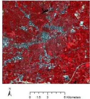
A heterogeneous area of 9.4 mi by 8.8 mi (15.1 km by 14.2 km) in central North Carolina, shown in Figure 7, was chosen as the study case for the proposed algorithm. It is from path/row 16/35 in Landsat and H/V11/5 in MODIS. The images of the study area were taken in 2001 when both Landsat 5 and Landsat 7 were in operation jointly, providing images at a nominal 8-day interval. For Landsat, the Surface Reflectance Climate Data Record (CDR) product was used. This is a new product released by USGS and NASA, which is atmospherically corrected to surface reflectance by the Landsat ecosystem disturbance adaptive processing system (LEDAPS) (Masek et al., 2006). This product has the benefit of providing quality assurance layers. These layers are used for masking clouds and cloud shadows. For MODIS, MODIS Terra daily data (MOD09GQ, 346 scenes) was downloaded. The proposed model was tested on the available bands in both Landsat and MODIS (i.e., the red bands). The Normalized Difference Vegetation Index (NDVIs) were also used in this test because the MODIS scenes include bands in the red and near infrared (NIR), and are inclined toward vegetation indices (Brooks et al., 2012). NDVI is used to monitor seasonal and interannual changes in plant phenology and biomass.

A preprocessing step was applied to both Landsat and MODIS images. Dark object subtraction, the subtraction of the smallest value in a band from every other value in that band, was applied to the Landsat images. Most of the processing was performed using R version 3.0.2 applying the spatial.tools library (Greenberg, 2014). For MODIS, resampling, subsetting, and reprojecting the images via the MODIS Reprojection Tool into Landsat scale and projection were applied (Dwyer et al., 2006).

Wavelet decompositions were performed, using MATLAB 2013b, on Landsat images at times . Low-frequency components of the Landsat images were merged with the MODIS images using (5), as described in the previous section. High-frequency components of the Landsat images were combined using (6). The final images were obtained by performing inverse wavelet transform on the prepared low-frequency and high-low-frequency components.

To assess the performance of the proposed technique, a number of existing Landsat images have been estimated using the proposed technique. Two measures of accuracy were used for the quantitative assessment; the coefficient of determination (R2) and the Root Mean Squared Error (RMSE).

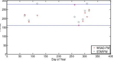
Figure 8 shows the results of prediction at times tp along with

the actual Landsat images for the red band (band 3). Figure 9 shows the results of prediction at times tp along with the actual

Landsat images for the NDVI. Figure 10 and Figure 11 show the computed R2 and RMSE values for all of the estimated red band images respectively, along with corresponding values that were obtained using STARFM. STARFM source code under Linux was obtained from NASA (LEDAPS tools). The default values in the input files were used. Figure 12 and Figure 13 also show the R2 and RMSE for the estimated NDVI images respectively. As shown in these figures the R2

and RMSE results

are very promising. To assess the correlation between the predicted and the actual NDVI pixel values, 100 pixels were randomly selected. The results of this experiment are shown in Figure 14, Figure 15 and Figure 16.

tp = 69

tp =277

tp =209

(a) (b)

Figure 6. Proposed fusion model using two time instants, t1 and t2, to estimate a Landsat image at intermediate time tp.

Coarse Resolution

Date tp

Landsat

Date t p

MODIS

Inverse Transform

Estimation of High-Frequency

Components

Date t 1

Landsat

Date t 2

Landsat

Mixing of Low-Freq. Components

Level M

Wavelet Transform

Date t 2

MODIS

Date t 1

MODIS

Fine Details Fine

Details

Fine Details

Figure 7. The study area shown in 4/3/2 combination, Greensboro, North Carolina, USA. UL/LR (X,Y): (601575, 3998835) / (616665, 3984645).

Figure 8. Comparison of Landsat images with predicted results at fine spatial resolution. (a) Red bands from actual Landsat images at times tp. (b) Predicted Landsat images. The International Archives of the Photogrammetry, Remote Sensing and Spatial Information Sciences, Volume XL-1, 2014

tp = 69

200 300 400 500 600 700 800

100

Figure 11. RMSEvalues for predicted red bands of Landsat images at time tp.

Figure 9. Comparison of actual NDVI images with predicted results at fine spatial resolution. (a) Actual NDVIs at times tp. (b) Predicted NDVI images.

5. CONCLUSION

A Wavelet-based Spatiotemporal Adaptive Data Fusion Model (WSAD-FM) has been proposed. The main idea of the model is to decompose several available images into different levels of detail, and then treat each level separately when combining the data into a single predicted image. The model was tested on MODIS and Landsat images to predict the Landsat images that were assumed to be unavailable. For validation purposes, images were produced that correspond to existing Landsat images. We observed R2 values in the range 0.70 to 0.92 for estimated Landsat images in the red band, and 0.62 to 0.89 for estimated NDVI images. These results demonstrate that the model shows promise, and it merits further investigation.

The novelty of this approach is two-fold. On one hand, unlike STARFM, the proposed technique treats the images at different levels of detail. Furthermore, unlike some Fourier-based approaches, WSAD-FM is not “data hungry” in the sense that lengthy temporal sequences of images are not needed in order to do the prediction. For the results shown here, a total of 3 MODIS images and 2 Landsat images were used to predict a single Landsat image. Ultimately, although not demonstrated here, the proposed approach can rely on images from only one additional instant in time, whereas some Fourier-based approaches require an entire year of data in order to perform the prediction.

ACKNOWLEDGEMENTS

Thanks to Dr. Evan Brooks, department of Forest Resources and Environmental Conservation, Virginia Tech, for his guidance during all the work. Thanks also to Dr. James Campbell and Dr. Yang Shao, department of Geography, Virginia Tech, for their guidance in early stage of the work.

REFERENCES

Brooks, E. B., Thomas, V. A., Wynne, R. H., and Coulston, J. W., 2012. Fitting the multitemporal curve: a Fourier series approach to the missing data problem in remote sensing analysis, IEEE Transactions on Geoscience and Remote Sensing, 50(9): 3340−3353.

Campbell, J. B., and Wynne, R. H., 2011. Introduction to Remote Sensing (5th edition), New York: Guilford.

Coifman, R. R., Meyer, Y., and Wickerhauser, M. V., 1992. Wavelet analysis and signal processing. In Ruskai M. B., Beylkin, G., Coifman, R. (Eds.), Wavelets and their Applications. 153−178. Jones and Bartlett (Boston).

Dwyer, J., and Schmidt, G., 2006. The MODIS reprojection tool. In Qu, J. J., Gao, W., Kafatos, M., Murphy, R. E., and

Salomonson, V. V. (Eds.), Earth Science Satellite Remote Sensing: Data, Computational Processing and Tools. 162-177. Springer-Verlag and Tsinghua University Press.

Gabor, D., 1946. Theory of communication, Journal of the Institute of Electrical Engineers, 93: 429–457.

Gao, F., Masek, F. J., Schwaller, M., and Hall F., 2006. On the blending of the Landsat and MODIS surface reflectance: predicting daily Landsat surface reflectance, IEEE Transactions on Geoscience and Remote Sensing, 44(8): 2207−2218.

Gao, R. X., and Yan, R., 2010, Wavelets: Theory and Applications for Manufacturing, Springer Science & Business Media.

Garguet-Duport, B., Girel, J., Chassery, J., and Pautou, G., 1996. The use of multiresolution analysis and wavelets transform for merging SPOT panchromatic and multispectral image data. Photogrammetric Engineering & Remote Sensing, 1057-1066.

Greenberg, J. A., 2014. Spatial.tools: R functions for working w ith spatial data. R package version 1.4.8. http://CRAN.R-projec t.org/package=spatial.tools.

Hansen, M. C., Roy, D. P., Lindquist, E., Adusei, B., Justice, C. O. and Altstatt, A., 2008. A method for integrating MODIS and Landsat data for systematic monitoring of forest cover and change in the Congo Basin. Remote Sensing of Environment, 112(5): 2495–2513.

Hilker, T., Wulder, M. A., Coops, N. C., Linke, J., McDermid, G., Masek, J. G., Gao, F., and White, J. C, 2009a. A new data fusion model for high spatial- and temporal-resolution mapping of forest disturbance based on Landsat and MODIS. Remote Sensing of Environment, 113(8): 1613–1627.

Hilker, T., Wulder, M. A., Coops, N. C., Seitz, N., White, J. C., Gao, F., Masek, J. G., and Stenhouse, G., 2009b. Generation of dense time series synthetic Landsat data through data blending with MODIS using a spatial and temporal adaptive reflectance fusion model. Remote Sensing of Environment, 113(9): 1988– 1999.

LEDAPS Tools website. [Online]. Available: http://ledaps.nascom.nasa. gov/tools/tools.html.

Mallat, S., 1989. A theory for multiresolution signal decomposition: The wavelet representation, IEEE Transactions on Pattern Analysis and Machine Intelligence, 11(7): 674-693.

Masek, J. G., Vermote, E. F., Saleous, N. E.,Wolfe, R., Hall, F.G., Huemmrich, K. F., Gao, F., Kutler,, J. and Lim, T.-K., 2006. A Landsat surface reflectance dataset for North America, 1990–2000. IEEE Geoscience Remote Sensing Letters, 3(1): 68–72.

Potapov, P., Hansen, M. C., Stehman, S. V., Loveland, T. R., and Pittman, K., 2008. Combining MODIS and Landsat imagery to estimate and map boreal forest cover loss. Remote Sensing of Environment, 112(9): 3708–3719.

Shi, W., Zhu, C., Zhu, C., and Yang, X., 2003. Multi-band wavelet for fusing SPOT panchromatic and multispectral

images”. Photogrammetric Engineering & Remote Sensing, 69(45): 513-520.

Weng, Q., Fu, P., and Gao, F., 2014. Generating daily land surface temperature at Landsat resolution by fusing Landsat and MODIS data. Remote Sensing of Environment, 145: 55-67.

200 300 400 500 600 700 800 200

Zhang, W., Li, A.N., Jin, H.A., Bian, J.H., Zhang, Z.J., Lei, G.B., Qin, Z.H., and Huang, C.Q., 2013. An enhanced spatial and temporal data fusion model for fusing Landsat and MODIS surface reflectance to generate high temporal Landsat-like data. Remote Sensing. 5: 5346–5368.

Zhu, X. L., Chen, J., Gao, F., Chen, X. H., and Masek, J. G., 2010. An enhanced spatial and temporal adaptive reflectance fusion model for complex heterogeneous regions. Remote Sensing of Environment, 114(11): 2610–2623.