ABOUT THE APPLICATIONS OF UNMIXING-BASED DENOISING FOR
HYPERSPECTRAL DATA
Daniele Cerra, Rupert M ¨uller, Peter Reinartz
German Aerospace Center (DLR)
Muenchner Strasse 20, Oberpfaffenhofen, 82234 Wessling, Germany [email protected], [email protected], [email protected]
KEY WORDS:Hyperspectral remote sensing, denoising, spectral unmixing
ABSTRACT:
Unmixing-based Denoising is a recently defined method which exploits spectral unmixing to recover bands characterized by a low Signal-to-Noise Ratio in a hyperspectral scene. The output of the unmixing process, which aims at decomposing each image element in signals typically related to pure materials, is inferred into the pixelwise reconstruction of a given band, ignoring the residual vector which is mainly characterized by undesired atmospheric influences and sensor-induced noise. The reconstructed images exhibit both high visual quality and reduced spectral distortions. This paper analyses the main problems that must be taken into account when applying this technique to real data. Special attention is given to the reference spectra used in the linear mixing model, which should be selected in order to keep the informational content of a given band unaltered in the reconstruction step.
1 INTRODUCTION
The spectral range characterizing data acquired by state-of-the-art hyperspectral sensors mostly spans the frequencies between 400 nm and 2500 nm. Some bands are related to frequencies which are mostly absorbed by the atmosphere, such as the ones in the near-ultraviolet and blue portions of the spectrum. As the sensor receives a low energy signal at such frequencies, these are typically characterized by a low Signal to Noise Ratio (SNR). On the other hand, at other frequencies sensor-induced noise be-comes predominant. As a consequence, these bands are often discarded in a preprocessing step common to most practical ap-plications. For some tasks, it would be desirable to keep such spectral information to better estimate some specific parameters from the data.
Spectral unmixing (Bioucas-Dias et al., 2012) and denoising of hyperspectral images (Renard et al., 2008) have always been re-garded as separate problems. By considering the physical prop-erties of a mixed spectrum, Unmixing-based Denoising has been recentely introduced in (Cerra et al., 2013b) as a methodology representing any pixel as a linear combination of reference spec-tra in a hyperspecspec-tral scene. As the residual vector from the un-mixing process is largely due to atmospheric interferences and instrument-induced noise, we can reconstruct each pixel ignoring the residual vector, and along with it most of the noise affecting each pixel.
As the quality of the denoised image will greatly depend on the adopted mixing model, distortions introduced by imperfections in the model should be kept to a minimum, and several problems arise when applying this technique to real data. To begin with, noise may be present in the very spectra used as a basis for spec-tral unmixing: to avoid this, spectra which are similar accord-ing to given criteria can be averaged to reduce noise influences. Furthermore, different samples of the same material may present subtle differences in terms of spectral response, which should be captured in the model. Finally, it is important to use a set of spec-tra which allows a complete representation of the informational content of a given band in a scene. This paper proposes an algo-rithm to tackle this problem by iteratively adding spectra to the model: these are chosen according to the distortions in the re-constructed image, whenever these deviate significantly from the
typical random noise distribution. Experiments show that the pro-posed method can effectively retrieve information from corrupted bands characterized by a low SNR which are usually discarded, and could be useful to derive indices and parameters for specific applications.
The paper is structured as follows. Section 2 introduces Unmixing-based Denoising, while Section 3 illustrates the main challenges faced when using this algorithm in practical applications and how to tackle them. We conclude in Section 4.
2 UNMIXING-BASED DENOISING
The Unmixing-based Denoising (UBD) is a simple procedure which can be described as follows. Given a training dataset con-tainingn spectra, homogeneous to some degree, from each of kmaterials, a set of reference spectral signatures is defined as A = {x1, . . . , xi, . . . , xk}, where xi is the average of then
spectra belonging to materiali. Considering the mean value for a given reference spectrum reduces the presence of noise to a minimum, if each class is spectrally homogeneous. It must be re-marked that no assumption on the purity of the reference spectra is made. Then, for each hyperspectral image elementmwithp bands, withp << k, any unmixing procedure can be employed to decomposemin a combination of the reference spectra. If we assume this to be linear, we have:
m=
k
X
i=1
xisi+r, (1)
wheresiis the fraction or abundance of the reference spectrum
iinm, andrthe residual vector. The latter is mostly composed by errors in the model and noise. The errors derive from contri-butions related to materials not present inA, subtle variations of one or more materials inA, noise affecting the selected reference spectra, and non-linear mixing effects. The noise mostly comes from fluctuations in the pixel values due to the low SNR in some bands caused by atmospheric absorption, and instrument-induced noise. If the modelling errors inAare kept to a minimum, we ex-pect the noise term to be predominant in the residual vector for bands with low SNR, and we can derive a reconstructionmˆas: International Archives of the Photogrammetry, Remote Sensing and Spatial Information Sciences, Volume XL-1/W3, 2013
SMPR 2013, 5 – 8 October 2013, Tehran, Iran
Figure 1: Results on synthetic dataset with perfect model avail-able. From top left: (a) Band 40 from fractals synthetic dataset, heavily corrupted (SNR=10); (b) Band 40 without noise, ideal target; (c) Image (b) restored from (a) through UBD using the 9 original spectra; (d) Difference image obtained subtracting image (c) from image (a).
ˆ
m=
k
X
i=1
xisi, (2)
ignoringr, and along with it most of the noise affectingm. The described procedure is based on the assumption that if the contri-butions to the radiation reflected from a resolution cell are known, the value of noisy bands in that area can be derived by a combina-tion of the average values characterizing each component in that spectral range. The method needs as input a set of spectra that well characterize the scene, and is carried out independently for each pixel. As a certain homogeneity of the classes of interest is assumed, the method is expected to perform better on natural scenes where man-made objects (usually having a higher vari-ability) are not prevalent.
3 ITERATIVE REFERENCE SPECTRA SELECTION
The results obtained with the UBD method as illustrated in sec-tion 2 are dependent on the quality of the linear mixing model used. This section illustrates which results can be expected in an ideal case, and what can be done to mitigate the distortions introduced by errors in the adopted model. Special attention is given on how to include in the model all relevant spectra useful to recover a given band in a scene. In the following experiments we choose Non-negative Least Squares (NNLS) as unmixing al-gorithm (Bioucas-Dias et al., 2012).
3.1 An ideal case
In an ideal case, we have a perfect model comprising all the spec-tra related to materials within the scene, all such specspec-tra are noise-free and there are no subtle variations within a given material in terms of percentage of scattered energy at a given wavelength. To understand how the algorithm would work in such a case, we
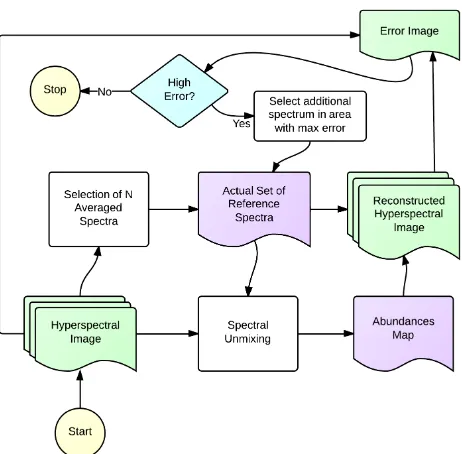
Figure 2: Workflow for the reported algorithm. The iterations up-date the set of reference spectra to be employed in the linear mix-ing model, keepmix-ing as much information as possible in a given noisy band and discarding all noise contributions.
apply UBD to a synthetic hyperspectral dataset by J. Plaza et al. (Plaza et al., 2012), available at (Plaza and Plaza, 2012). The dataset includes images composed by mixtures of 9 known pure spectral signatures with different noise levels (SNR ranging from 10 to∞). The spectra are selected from the USGS spectral li-brary (Clark et al., 2007), and the images are of size 100 x 100 pixels and have 221 bands between 0.4 and 2.5µm.
We consider the image with the worse SNR which is 10, and try to reconstruct the noise-free image from the noisy one, given the original noise-free spectra used to generate the target image, as in eq. 2. Results in fig. 1 show that, in spite of the high noise power, the target image is retrieved almost perfectly. As objective evaluation parameters we compute the average Normalized Root Mean Square Error (NRMSE) and the average Spectral Angle (SA) value, between the two images. The former is expressed in percentage as:
N RM SE(x, y) =
q Pn
i=1(xi−yi)2 n
xmax−xmin
, (3)
withxmaxandxminbeing the highest and lowest values assumed
byxrespectively, and the numerator the root of the mean squared error overnsamples. The SA, which measures the angle between two vectors representing two spectra. It is defined as the arcco-sine of the dot-product between two vectorsxandyas (Kruse, 1993):
SA(x, y) = cos−1
Pn i=1xiyi pPn
i=1xi2 pPn
i=1yi2
(4)
In this case after reconstruction the NMSE is 2.4%, while the average SA value is as low as 0.0346.
International Archives of the Photogrammetry, Remote Sensing and Spatial Information Sciences, Volume XL-1/W3, 2013 SMPR 2013, 5 – 8 October 2013, Tehran, Iran
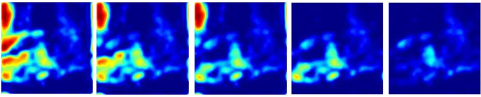
Figure 3: Sample steps from the iterative reference spectra selection. The reported images show the reconstruction error in a sample band at 434 nm, after a low-pass filtering carried out in the frequency domain. Red and dark blue areas correspond to high errors and to errors close to 0, respectively.
3.2 Real cases
In a real case the mixing model is generally unknown, along with the noise power and its distribution. Assuming non-linear mixing phenomenons to be negligible (Keshava and Mustard, 2002), the three main problems are: noisy reference spectra used as basis for the unmixing step, subtle variations of the same material which are not captured in the unmixing model, and missing spectra in the model. We briefly illustrate how to deal with these problems, with special attention to the last one.
The problem of noise presence in the basis used for the unmix-ing step can be strongly mitigated by considerunmix-ing each spectrum as the average of several similar signals. We assume the noise to be additive white Gaussian with zero mean, and signal-dependent noise to be negligible (Aiazzi et al., 2006). Whenever a spectrum is included into the model, the average values for each wave-length in a homogeneous area can be considered. This way, the mean of the noise in the considered spectra will be close to 0, and the typical values for a spectrum in bands affected by low SNR will be reliable. If no such area can be found, the average spec-trum can be computed using the spectra in the image which are the most similar to the initial one, and minimizes the SA between the two. Note that we are assuming that, for a given material, it is possible to identify several pixels in the image which are macro-scopically pure up to a certain degree. This also implies that we are not looking specifically for pure materials or endmembers, as also intimate mixtures represent valid candidates.
About the subtle variations within each material, nothing can be done if these cannot be expressed as linear combinations of the reference spectra used as basis for the unmixing step. This is a limitation of the method but it can be solved by considering different samples for the same material, which can in turn be mixed to obtain several intermediate states for the spectral re-sponse of any image element. This is done under the assumption that adding a spectrum which only slightly differs from one al-ready present in the model does not make the system unstable, i.e. does not cause one of the reference spectra to be linearly dependent from the others. This would introduce non-negligible numerical errors in the unmixing step, which requires the inver-sion of the matrix composed by the reference spectra.
This section mainly deals with the last of the described problems: finding all the spectra in the image which are needed to recon-struct an image discarding only its random noise component but keeping all relevant information in bands affected by low SNR. We could use any endmember extraction algorithm to retrieve the spectra which can at best represent the contents of a scene, but these would be driven by the full spectral information of a given image element, and would therefore implicitly give less impor-tance to variations in bands with low SNR. As these are exactly
the ones we want to retrieve, traditional endmember extraction algorithms are not fit to derive a model focused at keeping all the relevant information in these bands. Instead, we propose to use the following algorithm to retrieve the reference spectra which are useful to reconstruct one of such bands, for which the work-flow is sketched in fig. 2.
First of all, the set of reference spectra must be initialized. For this purpose, traditional algorithms which perform a rotation of the original data in a hyperplane with orthogonal components can be applied, such as Principal Components Analysis (PCA) (Kaewpijit et al., 2003) or Minimum Noise Fraction (MNF) (Am-ato et al., 2009) can be used. Selecting the extreme points in the space spanned by the first two dimensions in such spaces makes sure that the spectral information they convey is as uncorrelated as possible. In this way, 4 spectra can be selected to form the starting model for the unmixing algorithm.
Afterwards, an iterative reference spectra refinement method is carried out. In each step, the UBD algorithm is applied with the current mixing model, yielding a reconstructed image which will have at first high distortions with respect to the original one. At this point, the noisy band which is useful for a given application is selected, and an error image is generated by subtracting it from the original noisy band. The resulting error image will be com-posed by random noise and diffuse errors which are linked to the relevant information we lost by representing the image as a linear mixture of too few reference spectra. To separate these two com-ponents, the error image is filtered in the frequency domain with a Butterworth low-pass filter, yielding an error image containing only errors which are diffuse over an area. A filtered error image is of the kind reported in fig. 3. At this point, a new spectrum is selected from the area with maximum error and averaged over its neighbours (or similar pixels if the area is not homogeneous) to reduce noise contributions. The spectrum is added to the model and a new iteration takes place. As new spectra are added to the model, the error in the reconstructed image decreases: fig. 3 shows an example of the different outcomes of several itera-tions on the band at 434nmfrom a hyperspectral scene acquired by the HySpex sensor over the lake Starnberg in Germany. The original band is reported along with its final denoised version in figs. 4 and 5. In the processing the land and part of the boats have been masked out for computational efficiency reasons, as the main motivation for denoising this particular band is its util-ity in estimating the concentration of Coloured dissolved organic matter (CDOM) in natural waters, which is often carried out us-ing information at different wavelengths, given the low SNR of some bands in the blue portion of the spectrum (Kutser et al., 2005). After applying UBD, the retrieved CDOM parameters are closer to their actual values (Cerra et al., 2013a).
International Archives of the Photogrammetry, Remote Sensing and Spatial Information Sciences, Volume XL-1/W3, 2013 SMPR 2013, 5 – 8 October 2013, Tehran, Iran
Figure 4: Band 6 from the Starnberger lake dataset (434 nm).
4 CONCLUSIONS AND FUTURE WORK
Unmixing-based Denoising (UBD) is a supervised methodology for the recovery of bands characterized by a low Signal-to-Noise Ratio (SNR) in a hyperspectral scene. UBD reconstructs any pixel in a given band as a linear combination of reference spectra belonging to materials present in the scene. As the residual vector from the unmixing process is mostly composed by contributions of uninteresting materials, unwanted atmospheric influences and sensor-induced noise, this is ignored in the reconstruction pro-cess.
This paper focuses on how to include in the linear mixing model all relevant reference spectra to maximize the information which is kept in a given spectral band. The main problem when adopting this approach is deciding the stop criterion. In this work a thresh-old has been set as the maximum value which is allowed for an error image after a low-pass filtering in frequency, but several different criteria could be chosen. For example, spectra could be added until they are linearly independent regardless of the high-est value in the error image. Or the virtual dimensionality of the dataset could be estimated (Bioucas-Dias and Nascimento, 2008), and the process could stop when the same number of reference spectra is collected.
The proposed method could be applied to retrieve important in-formation in noisy bands for a wide array of practical applica-tions. Examples include: estimation of Leaf Clorophyll Content and vegetation stress for given kinds of crops, estimation of oil thickness in oil spill applications, estimation of CDOM in open waters, and vegetation damage severity index after forest fires.
REFERENCES
Aiazzi, B., Alparone, L., Barducci, A., Baronti, S., Marcoionni, P., Pippi, I. and Selva, M., 2006. Noise modelling and estima-tion of hyperspectral data from airborne imaging spectrometers. Annals of Geophysics.
Amato, U., Cavalli, R. M., Palombo, A., Pignatti, S. and Santini, F., 2009. Experimental approach to the selection of the com-ponents in the minimum noise fraction. IEEE Transactions on Geoscience and Remote Sensing 47(1-1), pp. 153–160.
Bioucas-Dias, J. and Nascimento, J., 2008. Hyperspectral sub-space identification. IEEE Transactions on Geoscience and Re-mote Sensing 46(8), pp. 2435 –2445.
Figure 5: Image in fig. 4 after denoising. Land and boats have been masked out.
Bioucas-Dias, J. M., Plaza, A., Dobigeon, N., Parente, M., Du, Q., Gader, P. and Chanussot, J., 2012. Hyperspectral unmixing overview: Geometrical, statistical, and sparse regression-based approaches. IEEE Journal of Selected Topics in Applied Earth Observations and Remote Sensing 5(2), pp. 354–379.
Cerra, D., M¨uller, R. and Reinartz, P., 2013a. Exploiting noisy hyperspectral bands for water analysis. In: Proc. 33rd EARSeL Symposium.
Cerra, D., M¨uller, R. and Reinartz, P., 2013b. Noise reduction in hyperspectral images through spectral unmixing. Geoscience and Remote Sensing Letters, IEEE PP(99), pp. 1–1.
Clark, R., Swayze, G., Wise, R., Livo, E., Hoefen, T., Kokaly, R. and Sutley, S., 2007. Usgs digital spectral library splib06a: U.s. geological survey. Digital Data Series.
Kaewpijit, S., Le Moigne, J. and El-Ghazawi, T., 2003. Auto-matic reduction of hyperspectral imagery using wavelet spectral analysis. IEEE Transactions on Geoscience and Remote Sensing 41(4), pp. 863 – 871.
Keshava, N. and Mustard, J., 2002. Spectral unmixing. IEEE Signal Processing Magazine 19(1), pp. 44 –57.
Kruse, F., 1993. The Spectral Image Processing System (SIPS) - Interactive Visualization and Analysis of Imaging Spectrometer Data. Remote Sensing of Environment 44, pp. 145–163.
Kutser, T., Pierson, D. C., Kallio, K. Y., Reinart, A. and Sobek, S., 2005. Mapping lake cdom by satellite remote sensing. Remote Sensing of Environment 94(4), pp. 535 – 540.
Plaza, J. and Plaza, A., 2012. Hypermix. http://www.hypercomp.es/hypermix.
Plaza, J., Hendrix, E. M. T., Garca, I., Martin, G. and Plaza, A., 2012. On endmember identification in hyperspectral images without pure pixels: A comparison of algorithms. Journal of Mathematical Imaging and Vision 42(2-3), pp. 163–175.
Renard, N., Bourennane, S. and Blanc-Talon, J., 2008. Denoising and dimensionality reduction using multilinear tools for hyper-spectral images. IEEE Geoscience and Remote Sensing Letters 5(2), pp. 138 –142.
International Archives of the Photogrammetry, Remote Sensing and Spatial Information Sciences, Volume XL-1/W3, 2013 SMPR 2013, 5 – 8 October 2013, Tehran, Iran