Evaluation of WGEN for generating long term
weather data for crop simulations
A. Soltani
a,∗, N. Latifi
a, M. Nasiri
baDepartment of Agronomy, Gorgan University of Agricultural Sciences, Gorgan, Iran bDepartment of Agronomy, Ferdosi University of Mashhad, Mashhad, Iran
Received 11 June 1999; received in revised form 20 December 1999; accepted 4 January 2000
Abstract
We evaluated the ability of the WGEN model to generate long term weather series in situations where the actual historic weather data record is only 3–10 years long. The series generated were used to simulate yield of irrigated and rainfed chickpea. To do this, four 100-year samples of weather data were generated for Tabriz, Iran. The WGEN parameters used to generate data were obtained from daily actual weather data of 3 (W3), 5 (W5), 7 (W7), and 10 (W10) recent years. The actual and generated weather series were each used as input to a chickpea crop model under irrigated and rainfed conditions at three planting dates. Results showed that the generated data are very similar to the actual data used for parameter estimation for all base periods tested. In comparison of the generated data and the historic data the means and the distributions of weather data variables differed significantly. However, with increasing the number of years used for parameter estimation of WGEN from 3 to 10, percent of significant differences were 38, 26, 17 and 13% for W3–W10, respectively. When generated weather data were evaluated as input to a chickpea crop model, simulated yields obtained using generated data were significantly different from that obtained using actual data in 50 and 8% of cases under irrigated and rainfed conditions, respectively. To generate data similar to long term historic data, a longer base period (>10 years) would be required for parameter estimation. However, when it is required that the generated data represent recent history rather than a long term period, the WGEN can be used as a reliable source of weather data even if it’s required parameters are obtained from only 3–10 years of actual historical weather data. © 2000 Elsevier Science B.V. All rights reserved.
Keywords:WGEN; Generating weather data; Crop simulation
1. Introduction
In agricultural science, crop simulation models are quantitative tools based on scientific knowledge that can evaluate the effects of climatic, edaphic, hy-drologic, agronomic, and genotypic factors on crop yield and stability (Boote et al., 1996). Such mod-els are used increasingly for genotype improvement
∗Corresponding author. Fax: +98-171-2220981/+ 98-171-2220438.
E-mail address:[email protected] (A. Soltani)
(Habekotte, 1997), environmental characterization and agro-ecological zonation (Aggarwal, 1993), es-timating production potential (Meinke and Hammer, 1995), quantifying climatic risk (Meinke et al., 1993), evaluating optimal management practices (Egli and Bruening, 1992; Muchow et al., 1994; O’Leary and Connor, 1998) and for predicting the effects of cli-matic change and clicli-matic variability on crop growth and yield (Matthews et al., 1997; Lal et al., 1998).
Long term weather data obtained at a specific site are usually required for simulation analyses. In regions with high climatic variability it is particularly
tant in order to assess effects of climatic variability. For the most commonly used models, this requires long term daily values of rainfall, solar radiation, max-imum and minmax-imum temperatures. However, many lo-cations do not have sufficient historical weather data. Many workers have recognized this problem, and this has led to the development of a range of weather generators such as WGEN (Richarsdon and Wright, 1984), SIMMETEO (Geng et al., 1986, 1988), TAM-SIM (McCaskill, 1990) and others (e.g. Larsen and Pense, 1982; Bristow and Campbell, 1984; Guenni et al., 1991) which can be used to generate weather data sets.
The quality of model output is related to the quality of weather data used as input. It follows that the test-ing of the sensivity of model output to the quality of generated weather data is an essential prerequisite for simulation analyses. Weather data is used in crop mod-eling not only to predict crop growth and development in response to environmental variables but also to flag catastrophic events such as heat stress, water deficit, frost damage and etc. Often such effects can only be assessed by using the weather data as input into the simulation models in question because model act as a data filter and integrate the effect of deviations of generated from actual data (Richardson, 1984; Meinke et al., 1995). Meinke et al. (1995) demonstrated how crop simulation models can be used to assess the ad-equacy and quality of weather data generation. They showed that model complexity did not appear to influ-ence model sensivity to differinflu-ences in environmental input data.
WGEN is a well-known and widely used stochastic weather generator that requires a number of parame-ters to generate a weather series at a site. This genera-tor has been incorporated into the WeatherMan (short for weather data manager, Pickering et al., 1994), an application program of Decision Support System for Agrotechnology Transfer (DSSAT) software (Tsuji et al., 1994). DSSAT is a collection of crop models and computer programs integrated into a single software package in order to facilitate the application of crop simulation models in research and decision making. This software is a product of the International Bench-mark Sites Network for Agrotechnology Transfer (IB-SNAT) project and is distributed over the world.
Richardson (1984) and Meinke et al. (1995) tested the WGEN output applied to crop simulation models
and showed that yields obtained using generated data were not significantly different from that obtained us-ing actual data. In these tests, parameters required by the model were obtained from long term actual data (longer than 10 years). However, we have found no report(s) showing the capability of WGEN for gener-ating long term data when model parameters are de-rived from relatively short term weather data, say 3–10 years. Thus, the objective of this study was the evalua-tion of the WGEN model for generating long weather series parameterized using short (3–10 years) records of actual data to derive a specific crop model.
2. Materials and methods
Chickpea (Cicer arietinumL.) is the most
impor-tant legume crop of Iran, and is sown on more than 50% of the total legume areas. The crop is predom-inately rainfed and only 10% is grown under irriga-tion (Sadri and Banai, 1996). Most chickpea growing areas of Iran which have cool and cold semiarid cli-mates with terminal drought stress (similar to that of Tabriz, the location chosen for this study) are located in north west (NW) of the country. Nearly 50% of to-tal chickpea production in Iran is concentrated in NW. Recently, a project was initiated to analyse the bio-physical limitations in chickpea production in Iran us-ing the crop simulation approach. However, at many locations long term weather data (more than 10 years) are not available to be used in the analysis. Therefore, we are forced to use a weather data generator to pro-vide long term weather series for use with the crop model.
2.1. The weather generation model
on whether the previous day was wet or dry. When a wet day is generated, the two-parameter gamma dis-tribution is used to generate the precipitation amount. For generating daily values of maximum and mini-mum temperature and solar radiation, the residual of the three variables are generated using a multivariate normal generation procedure that preserves the serial correlation and cross correlation of the variables. The final values of the three variables are determined by adding the seasonal means and standard deviations to the generated residual elements. For more details re-fer to Richardson (1981, 1984) and Richarsdon and Wright (1984).
2.2. The crop growth model
To evaluate the sensivity of crop models to observed versus generated data, we used the chickpea model of Soltani et al. (1999) with each of the observed and generated weather files. This model is similar to the models of Sinclair (1986), Amir and Sinclair (1991), and Hammer et al. (1995). The model is based on a daily time step and simulate crop growth and devel-opment as a function of temperature, solar radiation and water availability. Crop phenology is divided into two growth stages (before and after beginning seed growth), the duration of which are predicted based on daily temperature and water deficit. Leaf area devel-opment is calculated as functions of expansion and senescence of leaves. These functions are sensitive to temperature and water deficit. Daily biomass produc-tion is predicted from leaf area index, light extincproduc-tion coefficient and radiation use efficiency. Transpiration is calculated as a function of daily biomass produc-tion, transpiration efficiency coefficient and daily va-por pressure deficit. Daily biomass production and leaf growth decrease below potential values once the frac-tion of transpirable soil water (FTSW) declines below a threshold value (about 0.37). After the beginning of seed growth the accumulated biomass is partitioned into the grains, the rate of which depending on cli-matic conditions at and after beginning of seed growth. Soil evaporation, soil water drainage, and runoff are also calculated in the soil water balance sub-model. The model uses readily available weather and soil in-formation. The model was tested using independent data from a range of Iran’s environmental conditions.
In most cases, simulated grain yields were similar to that of observed yields. At this stage the model does not account for the effects of pests, diseases and soil fertility.
2.3. Procedure
Tabriz (38◦8′N, 46◦17′E and 1361 m above sea
level) was selected as the site for comparison of chick-pea model yield estimates made with actual weather data and data generated by WGEN as implemented in WeatherMan (Pickering et al., 1994). Precipitation and maximum and minimum temperature data were available for 30 years (1965–1995). Solar radiation data were calculated from sunshine hours and ex-traterrestrial radiation as outlined by Doorenbos and Pruitt (1977). With solar radiation data estimated, a complete 30-year daily data set of the required weather variables were available.
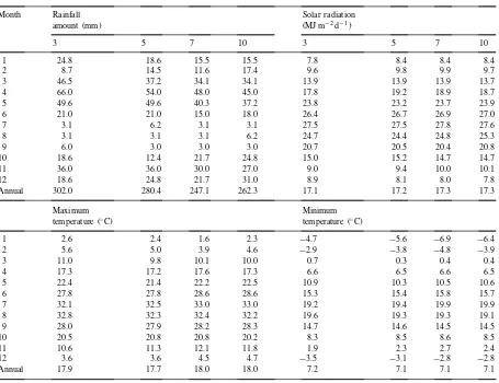
Four 100-year samples of weather data were gener-ated for Tabriz. The parameters used to generate data were obtained from daily weather data of 3, 5, 7, and 10 recent years as base periods (W3, W5, W7, and W10 thereafter). Monthly means of rainfall, solar ra-diation, maximum temperature and minimum temper-ature for 3, 5, 7 and 10 recent years are shown in Table 1. The actual and generated weather series were each used as input to the chickpea model. The same soil, cultivar and management inputs were used for all simulations. The soil that was chosen was sandy loam with a plant available water of 0.13 m3m−3, a depth
Table 1
Comparison of monthly rainfall amount, solar radiation, maximum and minimum temperatures averaged over recent 3, 5, 7 and 10 year periods
Month Rainfall Solar radiation
amount (mm) (MJ m−2d−1)
3 5 7 10 3 5 7 10
1 24.8 18.6 15.5 15.5 7.8 8.4 8.4 8.4
2 8.7 14.5 11.6 17.4 9.6 9.8 9.9 9.7
3 46.5 37.2 34.1 34.1 13.9 13.9 13.9 13.7
4 66.0 54.0 48.0 45.0 17.8 19.2 18.9 18.7
5 49.6 49.6 40.3 37.2 23.8 23.2 23.7 23.9
6 21.0 21.0 15.0 18.0 26.4 26.7 26.9 27.0
7 3.1 6.2 3.1 3.1 27.5 27.5 27.8 27.6
8 3.1 3.1 3.1 6.2 24.7 24.4 24.8 25.3
9 6.0 3.0 3.0 3.0 20.7 20.5 20.4 20.8
10 18.6 12.4 21.7 24.8 15.0 15.2 14.7 14.7
11 36.0 36.0 30.0 27.0 9.0 9.4 10.0 10.1
12 18.6 24.8 21.7 31.0 8.9 8.1 8.0 7.8
Annual 302.0 280.4 247.1 262.3 17.1 17.2 17.3 17.3
Maximum Minimum
temperature (◦C) temperature (◦C)
1 2.6 2.4 1.6 2.3 −4.7 −5.6 −6.9 −6.4
2 5.6 5.0 3.9 4.6 −2.9 −3.8 −4.8 −3.9
3 11.0 9.8 10.1 10.0 0.7 0.3 0.4 0.4
4 17.3 17.2 17.6 17.3 6.6 6.5 6.6 6.5
5 22.4 21.4 22.2 22.5 10.9 10.3 10.5 10.6
6 27.8 27.8 28.6 28.6 15.3 15.4 15.8 15.7
7 32.1 32.5 33.0 33.0 19.2 19.4 19.9 19.9
8 32.8 32.3 32.4 32.2 19.6 19.3 19.3 19.1
9 28.0 27.9 28.2 28.3 14.7 14.6 14.5 14.5
10 20.5 20.8 20.8 20.2 8.3 8.5 8.6 8.5
11 10.6 11.3 12.1 11.8 1.9 2.3 2.7 2.4
12 3.6 3.6 4.5 4.7 −3.5 −3.1 −2.8 −2.8
Annual 17.9 17.7 18.0 18.0 7.2 7.1 7.1 7.1
densities were 25 and 50 plants per m2under rainfed and irrigated conditions, respectively. Under irrigated conditions, the water balance sub-model was turned off. The management inputs were the same for each year of crop growth model runs. Thirty year simula-tions were made with the actual data and 100 years with the four series of the generated weather data. The daily water balance (only for rainfed conditions) and crop growth and yield were simulated for each year.
In each case, generated data were compared to the related base period data and to the entire 30-year length of record. The former tests indicate whether WGEN assumptions are valid and the latter tests show whether the base periods (3–10) are of sufficient length to adequately represent the entire data set.t-Tests were
used to compare the means of precipitation, number of wet days, solar radiation, maximum temperature, min-imum temperature, number of days with a maxmin-imum
temperature greater than 35◦C and number of days
with a minimum temperature less than 0◦C for each
month. Means of simulated yields (and some other crop related variables) using actual and four series of generated data were also compared byt-tests.
differences using Kolmogorov–Smirnov test. The Kolmogorov–Smirnov statistic is simply the max-imum absolute difference between the cumulative probability distributions of the two samples in ques-tion. The smaller the calculated test statistic, the smaller are the differences between the distributions in question. Statistical comparisons were performed using SAS (SAS Institute, 1989).
3. Results and discussion
3.1. Comparison of recorded historic and generated weather data
The mean rainfall amounts and mean number of wet days for each month of the year and for the an-nual totals are shown in Table 2 for the observed and generated data. The mean precipitation amounts from generated data differed significantly from the values obtained from the observed data for 4, 5, 3 and 3 of the 12 months for W3–W10, respectively. Rainfall of October–December and January–March has an im-portant role for increasing stored soil water and the successful growth of the crop under rainfed condi-tions is related to this stored water. The greatest dif-ferences between generated (W3–W10) and historic rainfall amount occurred in these months, specially in January and February. The discrepancy may be
cru-Table 2
Comparison of average monthly historic and generated rainfall amount and number of wet days for the four base periods used to parameterise WGEN
Month Rainfall amount (mm) Number of wet days
Observed W3 W5 W7 W10 Observed W3 W5 W7 W10
1 23.0 23.1 16.7∗ 13.2∗ 15.0∗ 8.6 11.0∗ 8.4 7.6 7.9
2 21.6 7.5∗ 10.7∗ 9.1∗ 14.4∗ 8.1 7.3 6.7 6.7 7.6
3 41.2 45.6 38.7 41.6 35.4 11.8 12.9 12.2 12.1 12.0
4 50.3 70.8∗ 50.2 46.3 47.3 11.4 11.6 10.0 10.1 11.1
5 44.0 46.3 55.0 43.5 41.8 11.3 11.2 14.3∗ 11.8 10.5
6 18.9 21.5 21.7 16.3 18.3 5.6 9.0∗ 8.5∗ 6.1 6.9
7 3.7 1.7 5.5 3.5 4.0 1.4 0.6∗ 1.5 1.6 1.7
8 3.5 2.2 3.0 3.1 5.5 1.2 1.7 1.4 1.1 1.7
9 8.5 4.7 2.5∗ 2.2∗ 1.8∗ 2.0 2.7 1.5 1.4 1.0
10 23.6 17.7 11.0∗ 18.7 28.4 6.7 3.2∗ 2.9∗ 3.7∗ 6.4
11 29.3 41.9∗ 41.8∗ 31.9 26.6 7.5 15.7∗ 11.8∗ 9.3 8.9
12 27.7 13.8∗ 25.7 23.8 35.2 8.2 3.8∗ 7.5 6.8 8.7
Annual 295.3 296.8 282.5 253.2 273.7 83.8 90.7 86.7 78.3 84.4
∗The observed mean and the generated mean are significantly different at the 1% level.
cial when applied to the crop model and discussed in latter section. The average number of wet days gen-erated for each month did not compare well with the long term averages for 6, 4 and 1 of the 12 months for W3, W5 and W7, respectively. The proper description of the occurrence of wet days by season is important, because the generation of solar radiation and maxi-mum temperature are conditioned on the occurrence of wet or dry days. Most of the differences between the recorded and the generated data that are shown in Table 2 were due to deviations of means of base peri-ods from the means of the historic period. For exam-ple, February rainfall are 7.5, 10.7, 9.1 and 14.4 mm for W3–W10 in comparison to 21.6 mm for the ob-served historic mean. For this month averages of rain-fall amounts are 8.7, 14.5, 11.6 and 17.4 mm for base periods of 3, 5, 7 and 10 years, respectively. There was a trend of reducing significant differences with lengthening of the base period used for parameter es-timation of the WGEN.t-Tests showed no significant differences between the generated data and their cor-responding base periods used for parameter estimation for precipitation and number of wet days (data not shown), suggested that model assumptions are valid.
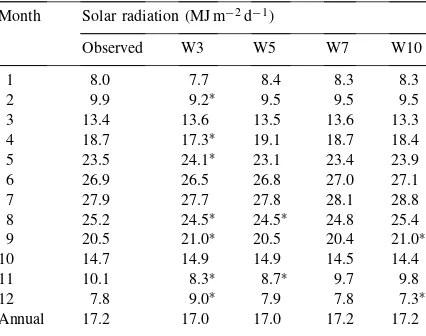
Table 3
Comparison of average monthly historic and generated solar radi-ation for the four base periods used to parameterise of WGEN
Month Solar radiation (MJ m−2d−1)
Observed W3 W5 W7 W10
1 8.0 7.7 8.4 8.3 8.3
Annual 17.2 17.0 17.0 17.2 17.2
∗The observed mean and the generated mean are significantly different at the 1% level.
respectively. The differences here were also due to deviations of means of base periods from the his-toric means. There were not significant differences between the generated data and their corresponding base periods for solar radiation (data not shown).
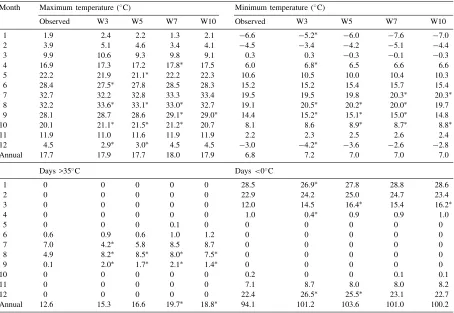
Table 4 shows a comparison between the historic and generated data (W3–W10) for maximum temper-ature, minimum tempertemper-ature, number of days with
maximum temperature greater than 35◦
C and num-ber of days with minimum temperature less than 0◦C
by month and annually. For maximum temperature, 35% of the time significant differences were observed between the generated data of W3, W5 and W7 and the historic data. For W10 only 1 of the 12 months has a significant difference. For minimum tempera-ture significant differences were detected between the recorded and the generated data in 5, 3, 4 and 2 of the 12 months, respectively. There was a tendency for lower significant differences with increasing of year number used to parameter estimation of the WGEN. The greatest differences between generated and actual number of days per month with a maximum tempera-ture greater than 35◦
C and the number of days with a
minimum temperature less than 0◦
C were occurred in the warmest and coldest months of the year, respec-tively, specially when WGEN’s required parameters were calculated from 3 years of recent actual data. The total annual number of days with a maximum
temperature greater than 35◦C were significantly
dif-ferent from the historic data for W7 and W10. The differences here between the generated data and their corresponding base periods data were not significant (data not shown).
The CDFs of the daily precipitation, solar radiation, maximum temperature and minimum temperature ob-tained from the generated and the recorded data were constructed and evaluated (data not shown). Statistical comparison using Kolmogorov–Smirnov test showed that all CDFs of generated maximum temperature and minimum temperature data and 50% of CDFs of gen-erated daily rainfall data differed significantly from the historic data (Table 5). There were not significant dif-ferences between simulated and actual solar radiation distributions in virtually all cases. The greater num-ber of years used to estimate the required parameters of WGEN did not affect on the number of significant differences.
gen-Table 4
Comparison of average monthly historic and generated maximum temperature, minimum temperature, number of days with maximum temperature greater than 35oC and number of days with minimum temperature less than 0oC for the four base periods used to parameterise
of WGEN
Month Maximum temperature (◦C) Minimum temperature (◦C)
Observed W3 W5 W7 W10 Observed W3 W5 W7 W10
1 1.9 2.4 2.2 1.3 2.1 −6.6 −5.2∗ −6.0 −7.6 −7.0
2 3.9 5.1 4.6 3.4 4.1 −4.5 −3.4 −4.2 −5.1 −4.4
3 9.9 10.6 9.3 9.8 9.1 0.3 0.3 −0.3 −0.1 −0.3
4 16.9 17.3 17.2 17.8∗ 17.5 6.0 6.8∗ 6.5 6.6 6.6
5 22.2 21.9 21.1∗ 22.2 22.3 10.6 10.5 10.0 10.4 10.3
6 28.4 27.5∗ 27.8 28.5 28.3 15.2 15.2 15.4 15.7 15.4
7 32.7 32.2 32.8 33.3 33.4 19.5 19.5 19.8 20.3∗ 20.3∗
8 32.2 33.6∗ 33.1∗ 33.0∗ 32.7 19.1 20.5∗ 20.2∗ 20.0∗ 19.7
9 28.1 28.7 28.6 29.1∗ 29.0∗ 14.4 15.2∗ 15.1∗ 15.0∗ 14.8
10 20.1 21.1∗ 21.5∗ 21.2∗ 20.7 8.1 8.6 8.9∗ 8.7∗ 8.8∗
11 11.9 11.0 11.6 11.9 11.9 2.2 2.3 2.5 2.6 2.4
12 4.5 2.9∗ 3.0∗ 4.5 4.5 −3.0 −4.2∗ −3.6 −2.6 −2.8
Annual 17.7 17.9 17.7 18.0 17.9 6.8 7.2 7.0 7.0 7.0
Days >35◦C Days
<0◦C
1 0 0 0 0 0 28.5 26.9∗ 27.8 28.8 28.6
2 0 0 0 0 0 22.9 24.2 25.0 24.7 23.4
3 0 0 0 0 0 12.0 14.5 16.4∗ 15.4 16.2∗
4 0 0 0 0 0 1.0 0.4∗ 0.9 0.9 1.0
5 0 0 0 0.1 0 0 0 0 0 0
6 0.6 0.9 0.6 1.0 1.2 0 0 0 0 0
7 7.0 4.2∗ 5.8 8.5 8.7 0 0 0 0 0
8 4.9 8.2∗ 8.5∗ 8.0∗ 7.5∗ 0 0 0 0 0
9 0.1 2.0∗ 1.7∗ 2.1∗ 1.4∗ 0 0 0 0 0
10 0 0 0 0 0 0.2 0 0 0.1 0.1
11 0 0 0 0 0 7.1 8.7 8.0 8.0 8.2
12 0 0 0 0 0 22.4 26.5∗ 25.5∗ 23.1 22.7
Annual 12.6 15.3 16.6 19.7∗ 18.8∗ 94.1 101.2 103.6 101.0 100.2
∗The observed mean and the generated mean are significantly different at the 1% level.
erated and recorded data and significant differences were rare. We examined this through analyses of out-puts of a chickpea crop model applied to generated and actual data.
3.2. Sensivity test using a chickpea crop model
Under rainfed conditions of NW Iran insufficient plant available soil water commonly overwrites any effects of variation in temperature and radiation. To eliminate this large influence of water availability on crop growth and hence on sensivity test, the chickpea crop model was run under irrigated (i.e. non-limiting water for plant growth) and rainfed conditions to eval-uate WGEN capability for generating temperature and radiation, and rainfall, respectively.
In the chickpea model the effects of non-optimal temperatures on plant growth is considered by multiplying radiation use efficiency (RUE) by a scalar
factor that has a value of 1 between 15–24◦C of
Table 5
Kolmogorov–Smirnov test statistics for the comparison of the dis-tribution of actual vs generated rainfall, solar radiation, maximum temperature and minimum temperature for the four base periods used to parameterise WGEN
W3 W5 W7 W10
Rainfall 0.018∗ 0.008 0.015∗ 0.007 Solar radiation 0.014 0.011 0.010 0.014 Maximum temperature 0.026∗ 0.032∗ 0.025∗ 0.022∗ Minimum temperature 0.021∗ 0.027∗ 0.024∗ 0.019∗
average daily temperature but declines linearly to 0 at 0 and 39◦C. The effect of higher temperature on
hastening crop phenology and leaf senescence is also incorporated. As indicated in Section 3.1, there were statistically significant differences between the gen-erated maximum temperature, minimum temperature, number of days with maximum temperature greater
than 35◦C and number of days with minimum
tem-perature less than 0◦C and the recorded ones during
April–August months which coincides with growing season of chickpea. It should be answered to this question whether these differences have significant influences on plant growth. To do this, during model simulations the number of days to maturity, number of days with average temperature between 15 and
24◦C (optimal days), number of days with average
temperature less than 15◦C (sub-optimal days) and
number of days with average temperature greater than
24◦C (supra-optimal days) were saved and compared
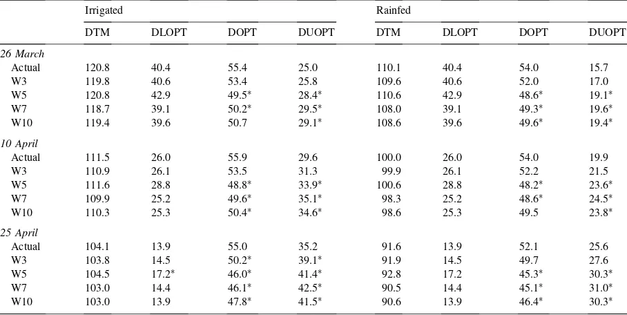
(Table 6). None of the base periods used had any influence on the simulated number of days to phys-iological maturity for all three sowing dates under
Table 6
Comparison of means of days to maturity (DTM), days with average temperature less than 15◦C (DLOPT), and days with average temperature between 15 and 24◦C (DOPT) and days with average temperature greater than 24◦C (DUOPT) simulated for three sowing dates under irrigated and rainfed conditions using the chickpea model with actual weather data and weather data generated with WGEN
Irrigated Rainfed
DTM DLOPT DOPT DUOPT DTM DLOPT DOPT DUOPT
26 March
Actual 120.8 40.4 55.4 25.0 110.1 40.4 54.0 15.7
W3 119.8 40.6 53.4 25.8 109.6 40.6 52.0 17.0
W5 120.8 42.9 49.5∗ 28.4∗ 110.6 42.9 48.6∗ 19.1∗
W7 118.7 39.1 50.2∗ 29.5∗ 108.0 39.1 49.3∗ 19.6∗
W10 119.4 39.6 50.7 29.1∗ 108.6 39.6 49.6∗ 19.4∗
10 April
Actual 111.5 26.0 55.9 29.6 100.0 26.0 54.0 19.9
W3 110.9 26.1 53.5 31.3 99.9 26.1 52.2 21.5
W5 111.6 28.8 48.8∗ 33.9∗ 100.6 28.8 48.2∗ 23.6∗
W7 109.9 25.2 49.6∗ 35.1∗ 98.3 25.2 48.6∗ 24.5∗
W10 110.3 25.3 50.4∗ 34.6∗ 98.6 25.3 49.5 23.8∗
25 April
Actual 104.1 13.9 55.0 35.2 91.6 13.9 52.1 25.6
W3 103.8 14.5 50.2∗ 39.1∗ 91.9 14.5 49.7 27.6
W5 104.5 17.2∗ 46.0∗ 41.4∗ 92.8 17.2 45.3∗ 30.3∗
W7 103.0 14.4 46.1∗ 42.5∗ 90.5 14.4 45.1∗ 31.0∗
W10 103.0 13.9 47.8∗ 41.5∗ 90.6 13.9 46.4∗ 30.3∗
∗Statistically significant difference.
irrigated and rainfed conditions. Significant differ-ences were observed between the generated data (W3–W10) and historic data for the number of opti-mal and supra-optiopti-mal days. In this respect, the lowest significant differences were observed for W3. Model output using recorded data showed that with delay in sowing date, percentage of sub-optimal and optimal days decreased but percentage of supra-optimal days increased. With the generated data of W3–W10 the same response was observed. Note that for 25 April planting date, each supra-optimal day has a more negative effect, because average daily temperatures are increased.
Table 7
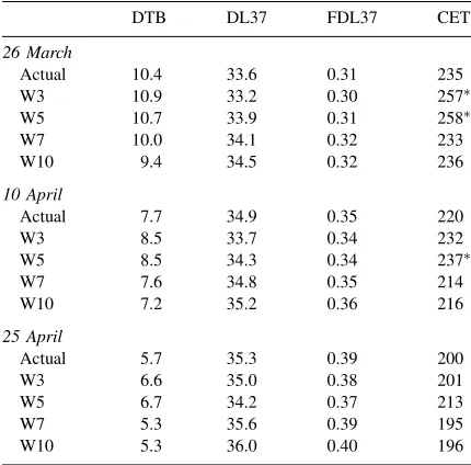
Comparison of means of days to terminal drought stress (DTB), days with fraction of transpirable soil water less than 0.37(DL37), ratio of DL37 to days to maturity (FDL37) and crop evapotranspi-ration (CET, mm) simulated for three sowing dates under rainfed conditions using the chickpea model with actual weather data and weather data generated with WGEN
DTB DL37 FDL37 CET
26 March
Actual 10.4 33.6 0.31 235
W3 10.9 33.2 0.30 257∗
W5 10.7 33.9 0.31 258∗
W7 10.0 34.1 0.32 233
W10 9.4 34.5 0.32 236
10 April
Actual 7.7 34.9 0.35 220
W3 8.5 33.7 0.34 232
W5 8.5 34.3 0.34 237∗
W7 7.6 34.8 0.35 214
W10 7.2 35.2 0.36 216
25 April
Actual 5.7 35.3 0.39 200
W3 6.6 35.0 0.38 201
W5 6.7 34.2 0.37 213
W7 5.3 35.6 0.39 195
W10 5.3 36.0 0.40 196
∗Statistically significant difference.
flowering as an origin) (DTB), days with FTSW less than 0.37 (DL37), ratio of DL37 to days to maturity (FDL37) and crop evapotranspiration (CET) using the generated and actual data inputted into the chickpea model and the results are presented in Table 7. Us-ing actual data, with delay in sowUs-ing date, terminal drought stress begins earlier and the crop experiences a greater number of days with FTSW less than 0.37 and FDL37 is increased. Simulations using generated data also showed the same response to sowing date, without any significant difference. With respect to considerable differences for winter rainfall between the generated and actual data (Table 2) and its influence on the stored soil water, the results of Table 6 seems questionable. However, because of the limited soil depth of the re-gion (100 cm, see Section 2.3) and its limited capacity for water storage, the differences were masked due to a higher water loss simulated using actual data. The differences could be of greater significance in other regions and climates or even in the same climate with deeper soils (although they are not common).
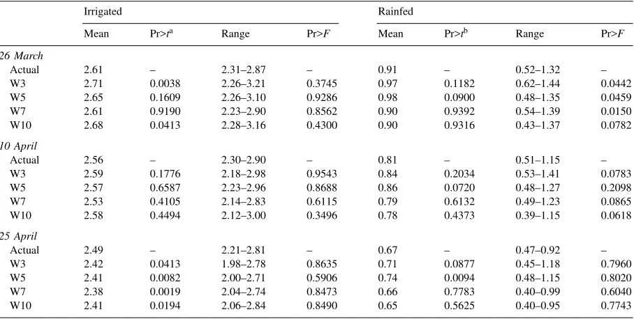
Table 8 shows simulated irrigated and rainfed yields at three sowing dates using actual and generated weather data. With actual weather data, irrigated yield
declined about 60 kg ha−1 (2% of 26 March yield)
for each 15-day delay in sowing date from 26 March. The same response was observed in simulated yields using W3–W10 weather data. At the two planting dates, i.e. 26 March and 10 April, there was no sig-nificant difference between irrigated yields obtained using actual weather data and those obtained using
W3–W10 weather data (p=0.01), with exception of
W3 at 26 March. However, at 25 April sowing date, simulated yields were significantly different at a prob-ability level of 0.05 from the simulated yields using actual weather data, because the growing season is moved into the summer months when the maximum differences between number of supra-optimal days using the generated and actual weather data occurred. Ranges of irrigated yields are generally similar and the F-test showed no significant difference between variances of simulated yields using actual weather data and W3–W10 weather data. The number of years used to estimate the required parameters of WGEN did not affect accuracy of the yield predictions.
Under rainfed conditions, simulated grain yield using actual weather data decreased by about 120 kg ha−1(13% of 26 March yield) per each 15-day
delay in sowing date (Table 8). Simulated yields us-ing generated weather data also showed the same response to sowing date. Means of yields obtained using actual weather data and W3–W10 were similar (with exception of W3 at 25 April). As compared to irrigated conditions delayed sowing date did not in-crease differences in yield, because water availability is an overriding factor under rainfed conditions and the differences between the generated and the historic data were not significant in this respect (Table 7). Yield ranges obtained from generated data were sim-ilar to those obtained using actual data, and F-test showed no significant difference between variances, with exception of W7 sown on 26 March. Under rainfed conditions, the number of data years used to parameterize WGEN also did not affect the conver-gence between simulated yield obtained using actual weather data and generated data.
Table 8
Comparison of means and ranges of chickpea grain yield (t ha−1) simulated for three sowing dates under irrigated and rainfed conditions
using the chickpea model with actual weather data and weather data generated with WGEN
Irrigated Rainfed
Mean Pr>ta Range Pr>F Mean Pr>tb Range Pr>F
26 March
Actual 2.61 – 2.31–2.87 – 0.91 – 0.52–1.32 –
W3 2.71 0.0038 2.26–3.21 0.3745 0.97 0.1182 0.62–1.44 0.0442
W5 2.65 0.1609 2.26–3.10 0.9286 0.98 0.0900 0.48–1.35 0.0459
W7 2.61 0.9190 2.23–2.90 0.8562 0.90 0.9392 0.54–1.39 0.0150
W10 2.68 0.0413 2.28–3.16 0.4300 0.90 0.9316 0.43–1.37 0.0782
10 April
Actual 2.56 – 2.30–2.90 – 0.81 – 0.51–1.15 –
W3 2.59 0.1776 2.18–2.98 0.9543 0.84 0.2034 0.53–1.41 0.0783
W5 2.57 0.6587 2.23–2.96 0.8688 0.86 0.0720 0.48–1.27 0.2098
W7 2.53 0.4105 2.14–2.83 0.6115 0.79 0.6132 0.49–1.23 0.0865
W10 2.58 0.4494 2.12–3.00 0.3496 0.78 0.4373 0.39–1.15 0.0618
25 April
Actual 2.49 – 2.21–2.81 – 0.67 – 0.47–0.92 –
W3 2.42 0.0413 1.98–2.78 0.8635 0.71 0.0877 0.45–1.18 0.7960
W5 2.41 0.0082 2.00–2.71 0.5906 0.74 0.0094 0.48–1.15 0.8020
W7 2.38 0.0019 2.04–2.74 0.8473 0.66 0.7783 0.40–0.99 0.6040
W10 2.41 0.0194 2.06–2.84 0.8490 0.65 0.5625 0.40–0.95 0.7743
aPr>t: Probability that a significanttvalue would occur by chance. bPr>F: Probability that a significantFvalue would occur by chance.
weather data, irrigated yields are between 2.34 and
2.75 t ha−1 in 80% of years (data not shown). Same
quantities were 2.34–2.82, 2.32–2.74, 2.28–2.72, and
2.31–2.79 t ha−1 for W3–W10, respectively. Grain
yield obtained using W7 weather data was greater than yield obtained using actual data for most of the years. Under rainfed conditions grain yields were be-tween 0.55 and 1.11 t ha−1in 80% of the years. Same quantities were 0.63–1.09, 0.65–1.10, 0.58–1.01, and
0.56–1.02 t ha−1 for W3–W10, respectively. Median
of yields were 2.55, 2.57, 2.53, 2.52, and 2.57 t ha−1
for actual data and W3–W10 under irrigated condi-tions and 0.75, 0.82, 0.85, 0.78, and 0.77 for actual data and W3–W10 under rainfed conditions, respec-tively. Statistical comparison showed that with one exception (W5 under rainfed conditions) all CDFs of simulated yield using generated data did not differed significantly from the simulated yield using recorded data (Table 9).
Briefly, in comparison of grain yields simulated using the generated solar radiation, maximum tem-perature and minimum temtem-perature and actual ones (i.e. irrigated yields), significant differences were
found in 50% of cases. Under rainfed conditions and using generated rainfall in addition to generated so-lar radiation, maximum temperature and minimum temperature, only in one out of 12 cases was a signif-icant difference (W5 for the 25 April planting date) observed in the comparison of simulated grain yields between W3–W10 against actual data. The uniformity was not due to capability of WGEN to generating weather data with adequate representation of actual data. It was resulted because considerable differences in rainfall amounts were masked by the limited soil depth (typical of the region) chosen for simulations.
Table 9
Kolmogorov–Smirnov test statistics for the comparison of the distribution of grain yield simulated using actual weather data vs generated weather data by base period used to parameterization of WGEN
W3 W5 W7 W10
Irrigated yield 0.129 0.049 0.123 0.119 Rainfed yield 0.163 0.210∗ 0.091 0.081
The longer base period used for parameter estimation of WGEN did not result in lower differences.
4. Concluding remarks
Our results show that
1. The WGEN’s generated data are very similar to the actual data used for parameter estimation for all base periods used (3, 5, 7 and 10 years). Therefore, WGEN assumptions are valid and the model is capable of representation of many of the characteristics that existed in the observed data. However, 3–10 years are not enough to adequately represent the historic data, because of the devia-tions of means of base periods from the means of the historic period.
2. In spite of similarity in trends and responses, sim-ulated yields obtained using generated data were significantly different from that obtained using ac-tual data in 50 and 8% of cases under irrigated and rainfed conditions, respectively. Under rainfed conditions differences were masked by the limited soil depth chosen for the simulations.
3. In many times it is better for the generated data to represent recent history rather than a long time pe-riod, particularly when the generated data are used to assess the risk of current decisions or represent future weather. In such cases, WGEN can be used as a reliable source of weather data for estimating crop yield.
Acknowledgements
The authors are thankful for the suggestions pro-vided by the referees and the regional editor which resulted in significant improvements.
References
Aggarwal, P.K., 1993. Agro-ecological zoning using crop simulation models: characterization of wheat environments of India. In: Penning de Vries, F.W.T., Teng, P.S., Metselaar, K. (Eds.), Systems Approaches for Agricultural Development. Kluwer Academic Publishers, Dordrecht, The Netherlands, pp. 97–109.
Amir, J., Sinclair, T.R., 1991. A model of water limitation on spring wheat growth and yield. Field Crops Res. 29, 59–69.
Boote, K.J., Jones, J.W., Pickering, N.B., 1996. Potential uses and limitations of crop models. Agron. J. 88, 704–771.
Bristow, K.L., Campbell, G.S., 1984. On the relationship between incoming solar radiation and daily maximum and minimum temperature. Agric. For. Meteorol. 31, 159–166.
Doorenbos, J., Pruitt, W.O., 1977. Guidelines for Predicting Crop Water Requirements, 2nd Edition. FAO Irrig. and Drain, Paper 24, FAO, Rome.
Egli, D.B., Bruening, W., 1992. Planting date and soybean yield: evaluation of environmental effects with a crop simulation model: SOYGRO. Agric. For. Meteorol. 62, 19–29.
Geng, S., Penning de Vries, F.W.T., Supit, I., 1986. A simple method for generating daily rainfall data. Agric. For. Meteorol. 36, 363–376.
Geng, S., Auburn, J.S., Brandstetter, E., Li, B., 1988. A program to simulate meteorological variables: documentation for SIMMETEO. Agronomy Progress Rep. 204, Department of Agronomy and Range Science, University of California, Davis, CA.
Guenni, L., Charles-Edwards, D., Rose, R., Braddock, R., Hogarth, W., 1991. Stochastic weather modelling: a phenomenological approach. Math. Comput. Simulation 32, 113–118.
Habekotte, B., 1997. Options for increasing seed yield of winter oilseed rape (Brassica napus L.): a simulation study. Field Crops Res. 54, 109–126.
Hammer, G.L., Sinclair, T.R., Boote, K.J., Wright, G.C., Meinke, H., Bell, M.J., 1995. A peanut simulation model I. Model development and testing. Agron. J. 87, 1085–1093.
Knisel, W.G., 1980. CREAMS: a field scale model for chemicals, run off and erosion from agricultural management systems. Conservation Research Report 26, USDA, U.S. Gov. Print. Office, Washington, DC.
Lal, M., Singh, K.K., Rathore, L.S., Srinivasan, G., Saseendran, S.A., 1998. Vulnerability of rice and wheat yields in NW India to future changes in climate. Agric. For. Meteorol. 89, 101–114. Larsen, G.A., Pense, R.B., 1982. Stochastic simulation of daily climatic data for agronomic models. Agron. J. 74, 510–514. McCaskill, M.R., 1990. TAMSIM — a program for preparing
meteorological records for weather driven models. Tropical Agronomy Technical Memorandum No. 65, CSIRO, Div. of Tropical Crops and Pastures, Brisbane, 26 pp.
Matthews, R.B., Kropff, M.J., Horie, T., Bachelet, D., 1997. Simulating the impact of climate change on rice production in Asia and evaluating options for adaptation. Agric. Syst. 54, 399–425.
Meinke, H., Hammer, G.L., 1995. A peanut simulation model II. Assessing regional production potential. Agron. J. 87, 1093– 1099.
Meinke, H., Hammer, G.L., Chapman, S.C., 1993. A crop simulation model for sunflower II. Simulation analysis of production risk in a variable sub-tropical environment. Agron. J. 85, 735–742.
Meinke, H., Carberry, P.S., McCaskill, M.R., Hills, M.A., McLeod, I., 1995. Evaluation of radiation and temperature data generators in the Australian tropics and sub-tropics using crop simulation models. Agric. For. Meteorol. 72, 295–316.
environments II. Effects of planting date, soil water at planting, and cultivar phenology. Field Crops Res. 36, 235–246. O’Leary, G.J., Connor, D.J., 1998. A simulation study of wheat
crop response to water supply, nitrogen nutrition, stubble retention and tillage. Aust. J. Agric. Res. 49, 11–19. Pickering, N.B., Hansen, J.W., Jones, J.W., Wells, C.M., Chan,
V.K., Godwin, D.C., 1994. WeatherMan: a utility for managing and generating daily weather data. Agron. J. 86, 332–337. Richardson, C.W., 1981. Stochastic simulation of daily
precipitation, temperature, and solar radiation. Water Resources Res. 17, 182–190.
Richardson, C.W., 1984. Weather simulation for crop management model. ASAE, Paper No. 84–4541, New Orleans, LA, 11–14 December.
Richarsdon, C.W., Wright, D.A., 1984. WGEN: a model for generating daily weather variables. U.S. Dep. of Agric., Agric. Res. Service, ARS-8, 83 pp.
Sadri, B., Banai, T., 1996. Chickpea in Iran. In: Saxena, N.P., Saxena, M.C., Johansen, C., Virmani, S.M., Harris, H. (Eds.), Adaptation of Chickpea in the West Asia and North Africa Region. ICARDA, Aleppo, Syria, pp. 23–34.
SAS Institute, 1989. SAS/STAT User’s Guide, Version 6, 4th Edition. SAS Inst., Inc., Cary, NC.
Sinclair, T.R., 1986. Water and nitrogen limitations in soybean grain production I. Model development. Field Crops Res. 15, 125–141.
Soltani, A., Ghassemi-Golezani, K., Rahimzadeh-Khooie, F., Moghaddam, M., 1999. A simple model for chickpea growth and yield. Field Crops Res. 62, 213–224.