DISCUSSION AND PRACTICAL ASPECTS ON CONTROL ALLOCATION FOR A
MULTI-ROTOR HELICOPTER
Guillaume J. J. Ducard and Minh-Duc Hua
I3S, UNS-CNRS 06903, Sophia Antipolis, France
[email protected], [email protected]
KEY WORDS:Multi-rotor UAVs, Hexacopter, Control Allocation, Weighted Pseudo-inverse Matrix
ABSTRACT:
This paper presents practical methods to improve the flight performance of an unmanned multi-rotor helicopter by using an efficient control allocation strategy. The flying vehicle considered is an hexacopter. It is indeed particularly suited for long missions and for carrying a significant payload such as all the sensors needed in the context of cartography, photogrammetry, inspection, surveillance and transportation. Moreover, a stable flight is often required for precise data recording during the mission. Therefore, a high performance flight control system is required to operate the UAV. However, the flight performance of a multi-rotor vehicle is tightly dependent on the control allocation strategy that is used to map the virtual control vectorv= [T, L, M, N]T
composed of the thrust and the torques in roll, pitch and yaw, respectively, to the propellers’ speed. This paper shows that a control allocation strategy based on the classical approach of pseudo-inverse matrix only exploits a limited range of the vehicle capabilities to generate thrust and moments. Thus, in this paper, a novel approach is presented, which is based on a weighted pseudo-inverse matrix method capable of exploiting a much larger domain inv. The proposed control allocation algorithm is designed with explicit laws for fast operation and low computational load, suitable for a small microcontroller with limited floating-point operation capability.
1 INTRODUCTION
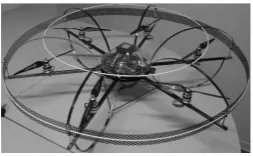
FUTURE generations of unmanned aerial vehicles (UAVs) will be capable of carrying tasks such as cartography, photogramme-try, surveillance, monitoring, inspection or transportation. To this end, new types of vehicles can be used, such as multi-rotor heli-copters, which are capable of lifting a significant payload while maintaining their flight stability. For example, the six-rotor heli-copter shown in Fig. 1 – called Hexaheli-copter – used in our Labo-ratory, can lift off a payload of about1kg. Therefore, the vehicle can be equipped with a selection of sensors and instruments to perform the desired task. This additional payload may signifi-cantly change the weight distribution and the flight performance of the vehicle. Robust flight controllers are necessary to safely
Figure 1: Hexacopter in use in the I3S Laboratory
operate the UAV, in particular in urban areas, despite uncertain-ties in the knowledge of the weight, the inertia matrix, the dynam-ics of the payload itself, and aerodynamic disturbances (Rudin et al., 2011). In addition, the hexacopter is an appealing plat-form to increase flight safety, since a certain level of stability can be maintained despite certain motor failure(s). In the case of a multi-rotor helicopter, the performance of the flight control sys-tem is strongly dependent on the control allocation strategy. It consists in computing each motor speed so as to produce the de-sired thrust and moments in roll, pitch, and yaw as shown in Fig. 2. Several methods for control allocation have been described in the literature: direct control allocation (Durham, 1993), daisy chaining (Buffington and Enns, 1996), and the linear program-ming method (Ikeda and Hood, 2000). In conventional methods
((Bodson, 2002), (Harkegard, 2003)), the control allocator solves the following (possibly underdetermined) constrained system of equations, which may be regarded as a mapping in the controlled systemg(δ(t)) = v(t), with the true actuator control signals δ(t) ∈ RN and N being the number of actuators. After lin-earization, the mapping equation may be rewritten in the standard formulation of the constrained linear control allocation problem:
Aδ(t) = v(t),
δi(t)≤ δi(t) ≤δi(t), with the constraints
δi(t) = max{δi, min, ρi, downTs+δi(t−Ts)},
δi(t) = min{δi, max, ρi, upTs+δi(t−Ts)}, whereδi,max, δi,minare theithactuator position limits, ρi,up andρi,downare theith actuator rate limits, andTs is the sam-pling time of the digital control system. Note that in the context of this work, actuators’ dynamics are not considered. The main technique these methods have in common is solving a constrained optimization problem. The pseudo-inverse redistribution method ((Bodson, 2002), (Jin, 2005)) is another technique, which makes use of a pseudoinverse computation of the control input matrix A. Although it does not always provide an optimal solution, it is usually faster than the other methods.
The greatest benefit of the control allocation approach is achieved in over-actuated systems. Using control allocation, the design of the control system can be separated into the derivation of the control laws and the design of a control allocator. This approach offers the following three advantages:
1. The actuator constraints, such as speed and speed-rate lim-its, can be taken into account. In case one actuator is sat-urated, the remaining actuators can be used to produce the desired control effort.
3. In cases of actuator failures, a supervision controller can re-configure the behavior of the control allocator in order to compensate for those failures, without the need for redesign-ing the control laws.
Multi-rotor
Figure 2: Control allocation
A literature survey shows that most of the control allocation tech-niques have mostly been applied to airplanes having redundant control surfaces. To our knowledge, control allocation has rarely been discussed for multi-rotor helicopters and in particular for an hexacopter as described in this paper.
In the case of multi-rotor helicopters, the control allocation prob-lem is summarized as follows:
1. given a virtual control input vectorvcmd= [T, L, M, N]⊤ cmd generated by the flight controller,
2. find the set of propeller speedsΩˆ := [ˆω2
1;· · ·; ˆωn2]⊤, where the number of propellers isn,
3. such thatvcmd=A ˆΩ, with the constraintsω2
min≤ωˆi2 ≤
ω2
max, ∀i, i= 1. . . n.
For multi-rotor vehicles, control allocation is classically done by:
1. computing the pseudo-inverse of the matrixAin Eq. (3), 2. saturating the computed propeller speeds in between the
min-imum and the maxmin-imum propeller speeds possible.
The key contributions of this paper are:
1. to show that a control allocation strategy based on the classi-cal approach of pseudo-inverse only exploits a limited range of the vehicle capabilities to generate thrust and moments, 2. a novel approach is presented which is based on a weighted
pseudo-inverse method capable of exploiting a much larger domain achievable inv,
3. and finally, the control allocation algorithm is formulated in terms of explicit laws for fast operation and low com-putational load, suitable for a microcontroller with limited computation capability (Ducard et al., 2006).
2 CONTROL ALLOCATION: PROBLEM DEFINITION
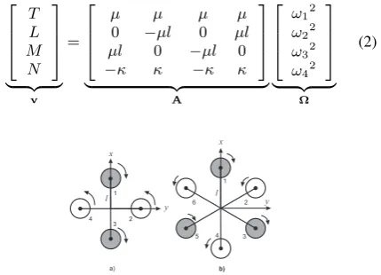
In the case of multi-rotor helicopters such as those represented in Fig. 3, control allocation consists in calculating each propeller speed to generate the desired total thrustT and the moments in roll, pitch and yaw,L,M,N, respectively. Consider a practical case of an helicopter withnrotors, where the speedωiof each motori(i = 1,2,· · ·, n) is lower and upper bounded by the positive numbersωminandωmaxrespectively, or equivalently
0< ω2min≤ω
The coefficientsµandκ(used below) characterize the efficiency of a propeller to generate thrust and yaw torque, respectively (Hamel et al., 2002). The arm-length of the vehicle isl.
2.1 Quadricopter Case
In the case of a quadricopter shown in Fig. 3, four motor speeds need to be computed. The mapping matrixAbetween propellers’ speed and the vectorvis shown in Eq. 2. Control allocation is done by computing the inverse of the matrixA, such that the commanded propeller speeds are calculated withΩc=A−1vc
.
Figure 3: Multi-rotor helicopter configurations: quadricopter in a), hexacopter in b)
2.2 Hexacopter Case
The hexacopter’s total thrust forceT and torque control inputs
L, M, N are related to the six motors’ speed by the following equation
which can be rewritten in a more compact form as
v=AΩ. (3)
We wish to determine the desired speedsωˆiof the six motors so thatv=AΩˆ, withΩ := [ˆˆ ω2
3 CONTROL ALLOCATION FOR HEXACOPTERS: CLASSICAL METHOD
3.1 Classical Pseudo-Inverse Matrix Method
and the desired motors’ speeds can be calculated according to
ˆ
Ω =A+v. (6)
3.2 Issues of the Classical Pseudo-Inverse Matrix Method
The most problematic issue of this classical pseudo-inverse ma-trix method is that it does not take the constraints given in Eq. (4) into account. For this issue, an existing popular solution con-sists in saturating the outputΩˆcalculated from Eq. (6) according to Eq. (4). However, due to the saturation of the outputΩˆ, the generated total thrustTˆ, roll torqueLˆ, pitch torqueMˆ, and yaw torqueNˆcan be dramatically different from the desired thrustT
and desired torquesL,MandN.
One verifies that the desired motors’ speedsωˆicalculated accord-ing to Eq. (6) satisfy the constraints (4) if and only if
Tminl≤ T l±2M∓µlκ−1N ≤Tmaxl
Tminl≤ T l∓ √
3L±M±µlκ−1N
≤Tmaxl
Tminl≤ T l∓ √
3L∓M∓µlκ−1N
≤Tmaxl
. (7)
In particular, whenN= 0, one verifies from (7) that
{
2|M| ≤min{(T−Tmin)l,(Tmax−T)l} √
3|L|+|M| ≤min{(T−Tmin)l,(Tmax−T)l}
.
For a given value of thrustT satisfying Eq. (1), all set-points {L, M}satisfying the above constraints form a symmetric cen-tered hexagon (see section 4.2.1). In the next subsection, we will show that the classical pseudo-inverse matrix method is very lim-ited in exploiting the capabilities of the vehicle. Moreover, we propose a novel weighted pseudo-inverse matrix method which improves significantly the admissible zone for the control torques
L, M, N.
4 CONTROL ALLOCATION FOR HEXACOPTERS: NEW PROPOSED WEIGHTED PSEUDO-INVERSE
MATRIX METHOD
4.1 General Formulation :
Let us introduce a diagonal weighting matrix
W :=diag([a;b;c;a;b;c]),wherea, b, care non-negative and satisfy the conditiona+b+c= 1.The weighted pseudo-inverse matrix proposed in the present paper is given by
A+W=WA⊤(AWA⊤)−
1 = 1
6µl
3al 0 2 −µlκ−1 3bl −√3 1 µlκ−1 3cl −√3 −1−µlκ−1 3al 0 −2 µlκ−1 3bl √3 −1−µlκ−1 3cl √3 1 µlκ−1
. (8)
The desired motors’ speedsωˆicalculated withΩ =ˆ A+Wvsatisfy
the constraints in Eq. (4) if and only if
Tminl≤ 3a T l±2M∓µlκ−1N ≤Tmaxl
Tminl≤ 3b T l∓ √
3L±M±µlκ−1N
≤Tmaxl
Tminl≤ 3c T l∓ √
3L∓M∓µlκ−1N
≤Tmaxl
. (9)
Now it matters to determine the appropriate set(a, b, c)and the domain of{T, L, M, N}such that the constraints given in Eq. (9) are satisfied. For the clarity of the presentation, let us first present our approach for the case where the desired yaw torque control is set to zero (N = 0). In this case, only the controls of
the thrustTand torquesL, Mare considered, and theadmissible zone1of
{L, M}will be characterized in function ofT in sec-tion 4.2. Then, in Secsec-tion 4.3 we extend the proposed approach for the case where the desired yaw torque control is chosen dif-ferent from zero (i.e.,N ̸= 0).
4.2 Case of Null Desired Yaw Torque Control, i.e.,N= 0: In this case, one easily verifies from Eq. (9) that
2|M| ≤min{(3aT−Tmin)l,(Tmax−3aT)l} |√3L−M| ≤min{(3bT−Tmin)l,(Tmax−3bT)l} |√3L+M| ≤min{(3cT−Tmin)l,(Tmax−3cT)l}
(10)
The constraints given in Eq. (10) indicate that for each set(a, b, c) and each commanded thrustT, the admissible values of the torque controlsL andM must stay inside a centered polygon, which can be a quadrilateral or a hexagon depending on the case. For instance, theclassical pseudo-inverse matrixis a particular case of the weighted pseudo-inverse matrix whena=b=c= 1/3. In this case the admissible zone of{L, M}is a symmetric cen-tered hexagon, which is named as “classical” admissible hexagon of{L, M}as shown in Fig. 8.
For a given value of thrustT, by varyinga, b, cunder the condi-tiona+b+c = 1and in view of Eq. (10), one observes that all possible admissible values of the set-point(L, M)fill a cen-tered hexagon which is bigger than the hexagon of the classical pseudo-inverse matrix case. In what follows, we will
• characterize the size of this “weighted” admissible hexagon of{L, M}in function ofT, and compare it with the “clas-sical” admissible hexagon of{L, M},
• propose a method to calculate the set(a, b, c)from a given set-point(L, M)which stays inside or on the borderlines of the weighted admissible hexagon of{L, M}.
4.2.1 Admissible Hexagon {L, M} in function ofT (with null desired yaw torque controlN = 0) This section is dedi-cated to define geometrically the shape of the admissible hexagon in terms of torques{L, M}for a given thrustT, when there is no yaw control. To this end, we first need to define the normalized variables for thrust and roll, pitch torque as follows:
e:=Tmin 3T , E:=
Tmax 3T ,L¯:=
L T l,M¯ :=
M
T l. (11)
In view of Eqs. (1) and (11), one hase≤1/3andE≥1/3; and Eq. (10) can be rewritten as
2|M¯| ≤3 min{a−e, E−a} |√3 ¯L−M¯| ≤3 min{b−e, E−b} |√3 ¯L+ ¯M| ≤3 min{c−e, E−c}
. (12)
Classical Case :
The case of control allocation via classical pseudo-inverse of the matrixAcorresponds to the situation where the coefficienta=
b=c= 1/3. In such a case, it is found from Eq. (12) that the maximum normalized roll torque that the vehicle can generate is
¯
Lclassical
max as follows:
¯
Lclassical
max =
{
(1−3e)/√3 if E+e≥2/3 (3E−1)/√3 if E+e <2/3, 1The termadmissible zonemeans that for any set-point(L, M)
which implies that the maximum actual roll torque achievable is
Lclassical
max =T lL¯classicalmax yielding
Lclassical
max =
(T−Tmin)l √
3 if T ≤
Tmax+Tmin 2 (Tmax−T)l
√
3 if T >
Tmax+Tmin 2
. (13)
Weighted Pseudo-inverse Case :
In the weighted pseudo-inverse matrix case, Eq. (12) yields that the maximum normalized roll torque that the vehicle can generate isL¯weighted
max as follows
¯
Lweighted
max =
√ 3(1−3e)
2 if E≥1−2e √
3(E−e)
2 if
1−e
2 ≤E <1−2e √
3(3E−1)
2 if E <
1−e
2
, (14)
which is equivalent toL¯weighted
max =
√ 3 2 α, with
α:= min(1−3e, E−e,3E−1). (15) Based on the result of Eq. (14) and the definition ofL¯in Eq. (11), the maximum actual roll torque achievable using the weighted pseudo-inverse matrix isLweighted
max as follows:
Lweightedmax =T lL¯ weighted
max =
√
3(T−Tmin)l
2 ifTmin≤T≤
Tmax+ 2Tmin 3 √
3(Tmax−Tmin)l
6 if
Tmax+2Tmin 3 < T≤
2Tmax+Tmin 3 √
3(Tmax−T)l
2 if
2Tmax+Tmin
3 < T ≤Tmax
.
(16)
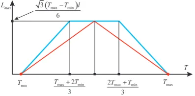
By noticing that the diameterDof the admissible centered hexagon of{L, M}is two times bigger than Lmax (i.e.,D = 2Lmax), one deduces from Eqs. (13) and (16) that the dimension (i.e., diameter) of the admissible hexagon of{L, M}in the proposed weighted pseudo-inverse matrix method is always larger than that of the classical pseudo-inverse matrix method (see Fig. 4). In-deed, Fig. 4 shows the comparison betweenLweighted
max andLclassicalmax in function of the thrustTand it appears in particular that
Lweighted
max = 3/2Lclassicalmax , for allT ∈
[
Tmin,Tmax+23 Tmin
]
orT ∈ [2Tmax+Tmin
3 , Tmax
]
. In addition, there exists a par-ticular value of the thrust, T = (Tmax+Tmin)/2, for which the two methods provide the same maximum roll torque, i.e.,
Lweighted
max =Lclassicalmax .
Figure 4: Comparison between the maximum roll torques achiev-able in the weighted pseudo-inverse matrix caseLweighted
max (blue line) and in the classical caseLclassical
max (red line) vs. thrustT
3D Characterization of the Admissible Zone{L, M}using the Weighted Pseudo-Inverse Matrix method :
Figure 5 shows the evolution of theweightedadmissible hexagon of{L, M}in function ofT (withN = 0). Its diameterD(T) increases linearly for T ∈ [Tmin,(Tmax+2Tmin)/3], remains constant forT∈[(Tmax+2Tmin)/3,(2Tmax+Tmin)/3], and de-creases linearly to zero forT∈[(2Tmax+Tmin)/3, Tmax]. From here, in a practical perspective, it is desirable to design hexa-copters such that the total thrust magnitudeT always remains in the interval[(Tmax+2Tmin)/3,(2Tmax+Tmin)/3].
Figure 5: Weighted admissible hexagon of{L, M}in function of
T(withN= 0)
Figure 6: Borderlines appellation of the weighted admissible hexagon of{L,¯ M¯}
Now for a given value ofT satisfying Eq. (1), let us characterize the borderlines of theweightedadmissible hexagon of{L, M}in the caseN= 0. To this purpose and in view of the definitions of
¯
L,M¯ in Eq. (11), it suffices to determine the borderlines of the weighted admissible hexagon of{L,¯ M¯}(see Fig. 6). From Eq. (14), the definition ofαin Eq. (15), and the hexagonal form, one easily deduces that :
• In thetop(equiv. bottom) line : L¯ ∈ [−√3α 4 ,
√ 3α 4
]
and ¯
M= 3α/4 (equiv.M¯ =−3α/4).
• In thetop-leftline:L¯∈[−√3α 2 ,−
√ 3α 4
]
,M¯=√3 ¯L+3α 2 .
• In thetop-rightline:L¯∈[√3α 4 ,
√ 3α 2
]
,M¯=−√3 ¯L+3α 2.
• In thebottom-leftline:L¯∈[−√3α 2 ,−
√ 3α 4
]
,M¯=−√3 ¯L−3α 2 .
• In thebottom-rightline:L¯∈[√3α 4 ,
√ 3α 2
]
,M¯=√3 ¯L−3α 2 .
Calculation of(a, b, c)in function ofT, L, M:
From a given set(T, L, M), we wish to calculate the weight-ing parametersa, b, cinvolved in the pseudo-inverse matrixA+W
thatLand M are chosen such that the set-point( ¯L,M¯) stays on the borderlines or inside the weighted admissible hexagon of {L,¯ M¯}specified previously. If this is not the case, one can eas-ily project the set-point( ¯L,M¯)onto this weighted admissible hexagon along the direction joining{L,¯ M¯}and the origin. In what follows, we deal withi) the case where( ¯L,M¯)stays on the borderlines, andii)the case where( ¯L,M¯)stays inside the weighted admissible hexagon of{L,¯ M¯}.
◮For each set-point( ¯L,M¯)on the borderlines of the admissible hexagon of{L,¯ M¯}, we propose to calculatea, b, cfor three pos-sible cases, so that the constraints given in Eq. (10) are satisfied, as follows :
◦Case 1 whereE≥1−2e, i.e.,Tmin≤T ≤Tmax+23 Tmin : • In thetopandbottomborderlines :
b= 1 +e • In thetop-leftandbottom-rightborderlines :
c=−1 + 5e • In thetop-rightandbottom-leftborderlines :
b=−1 + 5e
• In thetopandbottomborderlines :
b=2−E−e
• In thetop-leftandbottom-rightborderlines :
c=
• In thetop-rightandbottom-leftborderlines :
b=
• In thetopandbottomborderlines :
b= 1 +E • In thetop-leftandbottom-rightborderlines :
c= −1 + 5E • In thetop-rightandbottom-leftborderlines :
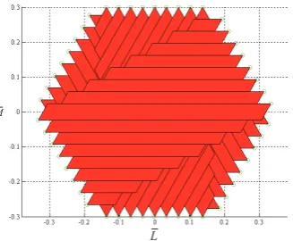
b= −1 + 5E which corresponds to the classical pseudo-inverse matrix case. The proposed expressions ofa, b, cfor the three above possible cases are quite tricky to get and are not presented in this paper due to space limitation. Essentially, they are based on the eval-uation on intersection points of six lines given in Eq. (12). For instance, these expressions ensure that when the reference set-point( ¯L,M¯) = ( ¯Lr,M¯r)moves continuously in the borderlines of the admissible hexagon{L,¯ M¯}, the variations of the weight-ing parametersa, b, care also continuous. Fig. 7 illustrates an example case whereE = 0.8ande = 0.2(i.e., Case 1). The green circles correspond to some reference set-points( ¯Lr,M¯r) moving clockwise in the borderlines of the admissible hexagon of{L,¯ M¯}, whereas the red quadrilaterals are zones limited by Eq. (12) with the weighting parametersa, b, ccalculated by the proposed expressions. We can see that each reference set-point ( ¯Lr,M¯r)coincides perfectly with a corner of the corresponding quadrilateral, which means that the constraints in Eq. (12) (i.e., Eq. (10)) are satisfied.
Figure 7: Reference set-points{L,¯ M¯}(blue circles) and corre-sponding admissible polygons{L,¯ M¯}(red quadrilaterals) with
a, b, cobtained.
◮Consider the case where the reference set-point( ¯L,M¯)is
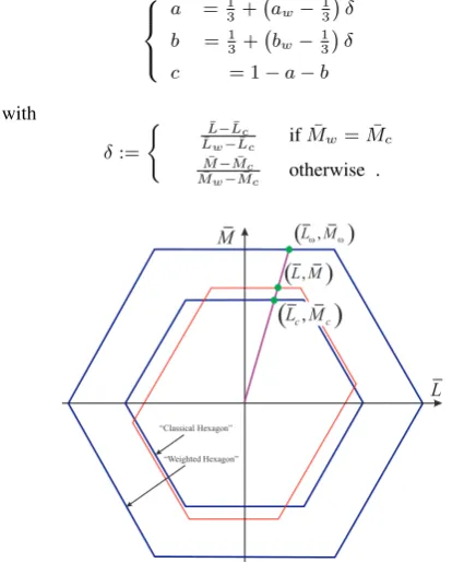
•When the set-point( ¯L,M¯)is inside or on the borderlines of the classical admissible hexagon, we seta=b=c= 1/3. •When the set-point( ¯L,M¯)stays outside theclassical admis-sible hexagonbut inside theweighted admissible hexagon, the following interpolation method is proposed (see Fig. 8). First, we project the reference set-point( ¯L,M¯)onto the borderlines of the classical and weighted admissible hexagons to obtain two set-points( ¯Lc,M¯c)and( ¯Lw,M¯w), respectively (see Fig. 8). Then, we apply the method previously proposed in order to calculate the parameters{a, b, c}for the set-point( ¯Lw,M¯w)staying on the borderlines of the weighted admissible hexagon. Let us de-note the corresponding values asaw, bw, cw. Finally, the desired parametersa, b, care calculated by interpolation as follows
a = 1 3+
( aw−13
) δ
b =1 3 +
(
bw−13)δ
c = 1−a−b
(17)
with
δ:=
{ L¯−L¯c
¯
Lw−L¯c if
¯
Mw= ¯Mc ¯
M−M¯c
¯
Mw−M¯c otherwise .
Figure 8: Interpolation method for the determination ofa, b, c
Fig. 8 illustrates an example case where the parametersa, b, care obtained by the proposed interpolation method. The red hexagon is the corresponding admissible zone of( ¯L,M¯)witha, b, c ob-tained and with the constraints in Eq. (12). It crosses the refer-ence set-point( ¯L,M¯), which means that the constraints in Eq. (12) (i.e., Eq. (10)) are satisfied. The proposed interpolation method ensures that the variations of the values ofa, b, care con-tinuous if the reference set-point( ¯L,M¯) varies smoothly over time. This is particularly important in practice since it ensures that the desired motors’ speedsωˆicalculated according toΩ =ˆ A+Wvvary also continuously if the control input vectorvis
con-tinuous in time.
4.3 Extension to the Case of Non-Null Desired Yaw Torque Control, i.e.N̸= 0:
In practice, it is desirable to maintain a certain control authority in yaw. However, in view of Eq. (9) the larger the value ofNthe smaller the dimension of the admissible zone of{L, M}. Thus, a compromise should be made. In the present paper, we propose to leave a certain control authority margin forN, i.e. |N| ≤Nmax whereNmaxshould not be too large. Define
TN:=µκ−1Nmax,
¯
Tmin:=Tmin+TN, T¯max=Tmax−TN.
Finally, instead of determining the admissible zone of{L, M} and the corresponding parametersa, b, cbased on the constraints given in Eq. (10), we consider now the following constraints
2|M| ≤min{(3aT−T¯min
)
l,(T¯max−3aT
) l}
|√3L−M| ≤min{(3bT−T¯min
)
l,(T¯max−3bT
) l}
|√3L+M| ≤min{(3cT−T¯min
)
l,(T¯max−3cT
) l}
. (18)
Eq. (18) is similar to Eq. (10) withTmin and Tmax replaced byT¯minandT¯max, respectively. From here, all the steps to de-terminea, b, ccan be proceeded exactly like in the case treated previously (i.e., case ofN= 0) but usingT¯minandT¯maxinstead ofTminandTmax, respectively.
5 CONCLUSIONS AND FUTURE WORK
This paper has shown new development in flight control system for multi-rotor helicopters. It is shown that a control allocation strategy based on the classical approach of pseudo-inverse matrix only exploits a limited range in the flight capabilities of the vehi-cle to generate the desired virtual control input vectorv. Thus, in this paper, a novel approach is proposed and is based on a weighted pseudo-inverse matrix method. It is capable of exploit-ing a significantly larger domain achievable inv. The presented control allocation algorithm is made of explicit laws for fast op-eration and low computational load. Future work deals with 1) the extension of the control allocation method to multi-rotors withn > 6propellers, 2) the on-line identification of the pro-pellers’ efficiency to generate thrust, and 3) dealing with control re-allocation in the case of one (or more) rotor failure(s).
REFERENCES
Bodson, M., 2002. Evaluation of Optimization Methods for Con-trol Allocation. AIAA Journal of Guidance, ConCon-trol, and Dy-namics 25(4), pp. 703–711.
Buffington, J. and Enns, D., 1996. Lyapunov Stability Analysis of Daisy Chain Control Allocation. AIAA Journal of Guidance, Control, and Dynamics 19(6), pp. 1226–1230.
Ducard, G., Geering, H. P. and Dumitrescu, E., 2006. Effi-cient Control Allocation for Fault Tolerant Embedded Systems on Small Autonomous Aircrafts. In: Proceedings of the 1st IEEE Symposium on Industrial Embedded Systems, Antibes, Juan les pins, France, pp. 1–10.
Durham, W., 1993. Constrained Control Allocation. AIAA Jour-nal of Guidance, Control, and Dynamics 16(4), pp. 717–725.
Hamel, T., Mahony, R., Lozano, R. and Ostrowski, J., 2002. Dy-namic modelling and configuration stabilization for an X4-flyer. In: IFAC World Congress, pp. 200–212.
Harkegard, O., 2003. Backstepping and Control Allocation with Applications to Flight Control. PhD thesis, Linkping University, Sweden.
Ikeda, Y. and Hood, M., 2000. An Approach of L1 Optimization to Control Allocation. In: AIAA paper 2000-4566.
Jin, J., 2005. Modified Pseudoinverse Redistribution Methods for Redundant Control Allocation. AIAA Journal of Guidance, Control, and Dynamics 28(5), pp. 1076–1079.