School of Earth and Space Exploration Arizona State University 550 E. Tyler Mall, Tempe AZ, 85287 [email protected], [email protected]
http://robotics.asu.edu/
Commission WG I/V
KEY WORDS:UAV, Photogrammetry, Structure from Motion, Terrain Mapping, Flight Planning, Camera Calibration
ABSTRACT:
We demonstrate a method for unmanned aerial vehicle based structure from motion mapping and show it to be a viable option for large scale, high resolution terrain modeling. Current methods of large scale terrain modeling can be cost and time prohibitive. We present a method for integrating low cost cameras and unmanned aerial vehicles for the purpose of 3D terrain mapping. Using structure from motion, aerial images taken of the landscape can be reconstructed into 3D models of the terrain. This process is well suited for use on unmanned aerial vehicles due to the light weight and low cost of equipment. We discuss issues of flight path planning and propose an algorithm to assist in the generation of these paths. The structure from motion mapping process is experimentally evaluated in three distinct environments: ground based testing on man-made environments, ground based testing on natural environments, and airborne testing on natural environments. Ground based testing on natural environments was shown to be extremely useful for camera calibration, and the resulting models were found to have a maximum error of 4.26 cm and standard deviation of 1.50 cm. During airborne testing, several areas of approximately 30,000m2were mapped. These areas were mapped with acceptable accuracy and a resolution of 1.24 cm.
1 INTRODUCTION
Three dimensional mapping is an extremely important aspect of geological surveying. The process to do this, however, often poses pragmatic challenges. Outdated methods such as walk-over surveying can create accurate, large-scale models. This type of surveying, however, requires a large amount of time and man-power. In addition, the resolution of these models depends upon the grid size of data points. A small increase in grid size requires a large increase in the number of data points, greatly lengthening the process.
Newer surveying methods can generate accurate, high resolu-tion models, however, they have their limitaresolu-tions. Light detec-tion and ranging (LiDAR) devices are able to make extremely accurate, high resolution models using short wavelength light pulses. These systems, until recently, were large and heavy, mak-ing them impossible to use on small unmanned aerial vehicles (UAVs) (Reineman et al., 2009). Although there are now com-pact LiDAR devices which are within the payload capabilities of small UAVs, these systems are still prohibitively expensive for many institutions. The cost of such systems and the inherently high risk of crashing makes the use of UAV-borne LiDAR de-vices impractical.
Photogrammetric techniques have been used for 3D mapping as early as 1849 (Birdseye, 1940). By 1904, the United States Ge-ological Survey (USGS) was utilizing photogrammetry for large-scale terrain mapping (Burtch, 2006). There are many different photogrammetric methods used for modeling, each having unique strengths and weaknesses. Stereo vision is one such technique used for modeling, however, it is not suitable for UAV-borne, large-scale, terrain mapping. Stereo vision uses the parallax be-tween two images to generate a 3D model (much like human vi-sion) (Matthies, 1992). This requires two separate cameras
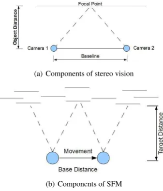
be-ing placed a known distance apart and bebe-ing triggered simul-taneously. The accuracy of stereo vision models is dependent upon the baseline-object distance ratio (Figure 1(a)). If the ob-ject distance is too great (with respect to the baseline distance), the images will not have enough parallax to generate an adequate model. In order to satisfy this requirement, the baseline distance must be increased or the object distance must be decreased. The baseline distance is limited, physically, by the size of the UAV. Therefore, in order to produce adequate models, the object dis-tance must be decreased. This is problematic for several reasons. Low altitude flights limit the ground image area (GIA). Small GIAs (relative to the total mapping area) cause drastically longer flights and larger amounts of data. This increases the time re-quired for data collection and image processing. Gathering data at low altitudes is also problematic for some UAVs due to the reduced flight speed necessary to prevent image blurring.
2 STRUCTURE FROM MOTION
Structure from motion (SFM) is a technique similar to stereo vi-sion which uses parallax between two images to create 3D models (Koenderink and Van Doorn, 1991). Instead of using two sepa-rate cameras, however, SFM uses a single, moving camera. The movement between sequential images creates enough parallax to infer 3D data (Figure 1(b)). The accuracy of these models de-pends upon a number of variables, however, the primary factors are the camera and lens. These aspects make SFM ideal for UAV-borne, large-scale terrain mapping.
(a) Components of stereo vision
(b) Components of SFM
Figure 1: Components of photogrammetry
in the models (Adamtech, 2010). SFM can be split into 5 main processes: camera calibration, data acquisition, feature detection, bundle adjustment, and 3D generation (Figure 2).
Figure 2: Flow chart of the structure from motion process
2.1 Camera Calibration
Camera calibration requires determining the interior properties of the camera and lens combination (Tsai, 1987). This greatly affects the quality of the model, therefore, it is crucial to perform a precise calibration. We will outline several factors which affect the calibration, issues encountered, and solutions to these prob-lems.
Focal length is one of the most important factors when perform-ing calibration. Therefore, the lens should be firmly attached to the camera, focused, and then fixed so that it cannot move. This prevents the focal length from changing due to handling, trans-portation, and vibrations from the UAV. When collecting images for SFM, there can be a variety of lighting conditions. In order to collect proper images, we must often alter the aperture setting. It is, therefore, beneficial to perform multiple calibrations with different aperture settings. Camera calibration accounts for the distortion occurring in images. Much of this distortion occurs near the edges of the photograph. When taking images for cali-bration, there should be a consistent number of features near the edges of the photograph (Figure 3). This will ensure that the cali-bration correctly accounts for the near-edge distortion. We found man-made environments such as rock gyms (shown in Figure 3) to be an ideal location to perform the camera calibrations. 2.2 Data Acquisition
Collecting appropriate data is imperative to the success of the SFM process. Familiarity with the SFM equipment and ade-quately preparing the UAV platform and flight path will facilitate
Figure 3: Image of Rock wall at Phoenix Rock Gym before and after feature detection (features marked with red)
satisfactory data collection. Recognition of which field condi-tions necessitate which camera settings (aperture, shutter speed, ISO) will prevent improperly exposed photos. Integrating SFM equipment into the UAV platform should be done in a manner which allows easy access yet protects the equipment from vi-brations, debris, and image pollution. This will decrease blur-ring in images and physically protect the camera and lens. UAV flight path planning will be discussed in more detail in Section 3, however, several general guidelines should be addressed. For the most accuracy and efficiency, images should be taken such that the camera-lens normal axis is perpendicular to the plane of the ground (Figure 4). Although this does not have to be precise, se-vere deviations (more than±15◦) from this will produce images
which are not useable. Sequential images should also attempt to carry a 60% overlap in the vertical direction and a 50% overlap in the horizontal direction. This was determined empirically to work with the 3DM software, although different overlap may be necessary for other software. An increase in overlap will still pro-duce functional images, however, less overlap is prone to cause issues later in the SFM process.
Figure 4: Ground imaging areas of proper and improper heli ori-entations
2.3 UAV Platform
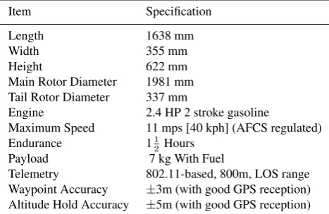
Figure 5: The SR30 platform with modifications and SFM
equip-Main Rotor Diameter 1981 mm Tail Rotor Diameter 337 mm
Engine 2.4 HP 2 stroke gasoline
Maximum Speed 11 mps [40 kph] (AFCS regulated)
Endurance 11
2 Hours
Payload 7 kg With Fuel
Telemetry 802.11-based, 800m, LOS range Waypoint Accuracy ±3m (with good GPS reception) Altitude Hold Accuracy ±5m (with good GPS reception)
Table 1: UAV Specifications
3 FLIGHT PATH PLANNING
Parallel line flight paths, also known as lawn mower flight paths, are widely used in aerial photography flights. This path forma-tion allows for consistent image overlap and data collecforma-tion in a uniform grid. However, these are not the only factors which con-tribute when planning a flight path. We sought to examine ele-ments which are key to aerial photography and propose a method for generating flight paths.
Terrain mapping with UAVs requires a flight path which accom-modates the desired ground sample distance (GSD), proper im-age overlap, and allows for appropriate imaging. In addition to the aerial photography aspect, UAV characteristics must also be taken into account. This means reducing flight distance and opti-mizing flight speed and altitude. If the turning radius of the UAV is limited, the flight path should also reflect this and minimize the number of difficult or impossible turns. These factors com-bine to make manual path planning a difficult task. Due to this complexity, we propose an algorithm which could assist with this planning.
The factors discussed above, while all significant, do not hold equal importance. When using UAVs as a tool for data collection, task optimization must be accommodated over flight optimization (to the extent that it does not cause risk to the UAV). For 3D map-ping, the model resolution or GSD is usually the limiting factor. In order to accommodate the desired resolution, we must restrict our above ground level (AGL) flight altitude. Maximum flight al-titude can be found using Equation 1. This, coupled with camera specifications, governs the ground imaging area (GIA) as related in Equation 2. Once the GIA has been determined, we can now begin planning the actual flight path.
h= rxgx
gx, gy= desired horizontal, vertical ground sample distance (m) θx= horizontal field of view
3.1 Path Planning Algorithm
Restricting the flight altitude effectively transforms flight path planning from a 3D problem to a 2D problem∗. This then leaves
us with the question of how to image the entire mapping area, and which path to travel to do so. The path planning problem can be thought of in two sections. First, the mapping area must be split into a finite number of identical rectangles. This represents the area being photographed. Identical rectangles are used because, assuming a constant altitude and minimal UAV pitch and roll, the ground imaging area of all photographs will be identical rectan-gles. Second, we must travel to the center of each rectangle in order to take the picture. Doing this in the shortest path avail-able is a version of the traveling salesman minimization problem (TSP). The traveling salesman problem is the task of visiting a finite number of locations via the shortest path (Kruskal, 1956) (Kirkpatrick et al., 1983).
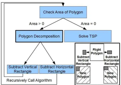
3.1.1 Polygon Decomposition Mapping areas are most often polygons. Those which are not, can be expanded, with minimal image waste, to become a polygon. Image waste refers to the amount of ground imaging area which does not lie within the de-sired mapping area. This reduces the imaging problem to a poly-gon decomposition problem. A polypoly-gon decomposition problem is the task of reducing a large polygon into a finite number of smaller polygons (Keil, 2000) (O’Rourke and Supowit, 1983). If we assume no vertical or horizontal overlap between images, the rectangles are of the same dimensions as the GIA. Similarly, as we increase the desired vertical and horizontal overlap, we re-duce the size of the rectangles proportionally. After determining the size of the rectangles (based upon desired overlap), we begin the polygon decomposition. This is done by arbitrarily starting at the top left corner of the polygon, subtracting a rectangle ori-ented vertically from the original polygon, subtracting a rectan-gle oriented horizontally from the original polygon, and recur-sively calling the algorithm on the two new polygons (Figure 6). Throughout the decomposition, we keep track of the decompo-sition history (whether each rectangle was oriented vertically or horizontally), the coordinates of the center of each rectangle, and the accumulated image waste. When the polygon is completely decomposed into rectangles, we can then sort the solutions based upon minimal image waste. Having determined the locations to take pictures, we can then move to the next portion of the algo-rithm, path minimization.
3.1.2 Path Minimization This portion of the path planning can be thought of as a traveling salesman problem, to which there are a variety of solutions. In the most basic case, we can use a purely Euclidean TSP solver. A Euclidean TSP solver mini-mizes the path based solely on the Euclidean metric (Papadim-itriou, 1977). This will provide a flight path with the shortest dis-tance. This is ideal for helicopter path planning for which there is no real disadvantage for turning. When path planning for UAVs with turning limitations, however, the algorithm should be modi-fied to include a cost for turning. We utilize an open source TSP solver provided by (Paris, 2008).
Figure 6: Flowchart of path planning algorithm - inset contains visual of polygon decomposition process
3.2 Algorithm Results
We have tested this process with multiple polygons in an attempt to test the robustness and accuracy of the algorithm. An image rectangle with dimension 3x4 units was chosen arbitrarily and used for all tests. For all test images, the inner black, solid-line rectangle represents the desired mapping area. The red, dashed line indicates the generated flight path, and the blue dashes show where pictures should be taken (Figures 7, 8, and 9). Starting with the most basic mapping area, we generated a flight path for a large rectangular area. As is suspected, the flight path is very similar to a lawn mower pattern (Figure 7(a)). Moving to a square area, we find a generated path which is slightly unusual (Figure 8(a)). This path, however, has a length of 42 units which is exactly the same as the lawnmower pattern shown in Figure 8(b). Polygons of various shapes and sizes have been tested with several solu-tions shown in Figures 7(b), 9(a), and 9(b). We also compared the actual flight paths flown while performing field testing in Las Cruces, New Mexico, with proposed the flight path (Figure 10). Direct comparison is challenging because the actual path had to be split into two flights due to camera issues. However, the algo-rithm does propose a shorter, alternate flight path. Although there is much room for improvement in the efficiency and robustness of this algorithm, this technique offers a starting point for flight path generation.
(a) Flight path for large rectangu-lar imaging area
(b) Flight path for large, irregular U-shaped imaging area
Figure 7: Predicted flight paths of polygons
4 EXPERIMENTAL EVALUATION
4.1 Ground Based Testing in Man-Made Environments
A Canon 5D (12.8 MP resolution and 35.8 x 23.9 mm sensor (Digital-Photography-Review, 2010)) with a 20mm lens was used to ground test the SFM process in a man-made environment. We chose to test the process at a local rock gym due to the high num-ber of distinct features and the structure complexity. An area of
(a) Proposed flight path for square imaging area
(b) Lawn Mower flight path for square imaging area
Figure 8: Predicted flight paths of polygons
(a) Flight path for small quadri-lateral
(b) Flight path for unusual poly-gon
Figure 9: Predicted flight paths of polygons
approximately 100m2was photographed, and distance
measure-ments were taken via manual methods in order to perform ac-curacy analysis. After generating the model, corresponding dis-tances were measured and compared to the actual disdis-tances (Ta-ble 2). We found the average error to be 0.85 cm with a stan-dard deviation of 1.50 cm and the maximum error to be 4.26 cm. The results were then compared to the predicted accuracies given by models from 3DM Analyst. Equations 3, 4, and 5 were used, where the planimetric accuracy is the error in the X and Y-directions and the depth accuracy is the error in the Z-direction (Adamtech, 2010). Using the given formulae, we predicted the total accuracy of this model to be 0.30 cm. Although the actual error of the model is very low, it does differ significantly from the prediction. We attribute this to the accuracy formulae not ac-counting for errors in camera calibration. Ultimately, the model produced was of high quality and accuracy, and it shows structure from motion to be a viable option for modeling.
σplan=σpixelγd
f (3)
σdepth=σpland
b (4)
σtotal= p
2σplan2+σdepth2 (5)
where:
σplan= planimetric accuracy (parallel to image plane) σpixel= estimated pixel accuracy
σdepth= depth accuracy (perpendicular to image plane) γ= pixel size d= target distance
f= focal length b= base distance
4.2 Ground Based Testing in Natural Environments
Figure 10: Actual (white and yellow) and proposed (red) flight paths of imaging area in Las Cruces, New Mexico (400 x 100 m)
Measu- Measured Model Meas- Differe- Percent rement Distance (m) urement (m) nce (cm) Error
1 1.321 1.320 -0.08 0.06
2 1.791 1.790 -0.07 0.04
3 2.057 2.080 +2.26 1.10
4 2.159 2.170 +1.10 0.51
5 2.210 2.210 +0.02 0.01
6 2.565 2.560 -0.54 0.21
7 2.756 2.740 -1.59 0.58
8 2.775 2.780 +0.51 0.18
9 2.908 2.920 +1.17 0.40
10 4.115 4.120 +0.52 0.13
11 4.204 4.220 +1.63 0.39
12 4.470 4.460 -1.04 0.23
13 5.334 5.340 +0.60 0.11
14 5.867 5.910 +4.26 0.73
15 6.166 6.200 +3.41 0.55
16 6.515 6.520 +0.49 0.08
17 7.252 7.270 +1.83 0.25
Table 2: Measurements from Phoenix Rock Gym and corre-sponding measurements from the resulting model
Camelback mountain near the Arizona State University. Many of these models suffered due to improper base-distance ratio (see Figure 1(b)) and shrubbery. An improper base-distance ratio of-ten does not provide enough parallax between images, while trees and shrubbery cause false positive feature matching.
The same equipment was tested again in Granite Dells, near Pres-cott, Arizona. This area allowed for better camera placement and, therefore, a better base-distance ratio. There was also a much clearer line of sight to the modeling target, providing more visi-bility of natural features. The models produced were of a much higher quality than those of the Camelback test site, however, ac-curacy analysis is still pending (Figure 11).
4.3 Airborne Testing in Natural Environments
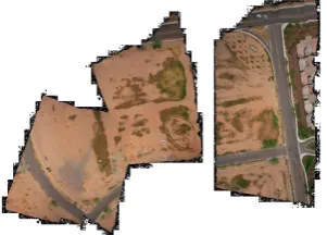
Airborne testing in a natural environment was first performed with the Canon T1i camera and 18-55 mm lens (manually fixed at 19 mm). This SFM equipment was tested in Las Cruces, New Mexico, and photographed an area approximately 400 x 100 m. Multiple models were generated (Figure 12), although some suf-fered from a variety of issues.
1. The variable focal length lens, although manually fixed at 19mm, had small changes due to vibrations which affected ac-curacy and prevented models from separate flights from being merged.
Figure 11: Model produced at Granite Dells (15 x 10 m) - (top) wireframe model - (bottom) same model with draped images
2. Due to unexpected UAV attitudes, improper flight paths, and camera backlog, overlap between some images was not adequate to produce models.
3. Blurring rendered some images unusable. This caused disrupts in the models and increased error.
Figure 12: Two views of 3D model of Las Cruces test site (400 x 100 m): (1) is topview of terrain (2) is view from approximately 60◦above horizon (insets show wireframe model and frame with
draped images)
Figure 13: Model generated at local Northgate flight field (350 x 200 m)
5 FUTURE WORK AND CONCLUSIONS
While we have shown that UAVs can be used as a platform to collect images for structure from motion mapping, there are sev-eral issues, pertaining to both UAV usage as well as the structure from motion process, which we plan on examining in the future. The path planning algorithm outlined above does offer a starting solution, however, there is much room for improvement. Incorpo-rating turning costs into the TSP solver as well as utilzing a TSP with neighborhoods (TSPN) solver could potentially offer more natural, UAV-friendly flight patterns (Dumitrescu and Mitchell, 2003). Due to GPS error, it is unlikely that a UAV will ever visit the exact location desired. Rather, there is an acceptable region which the UAV targets. In this same manner, there is an accept-able region, or neighborhood, from which the UAV can gather ap-propriate data. We believe that utilization of a TSPN solver would improve our algorithm and the resulting flight paths. Combining feature tracking with the SFM modeling process could help iden-tify moving objects in images and disregard them in the model-ing process. This would reduce false positive feature matchmodel-ing and, therefore, increase model accuracy. Lastly, using multiple vehicles to perform structure from motion modeling could allow
for this technique to model rapidly changing systems. Systems which are currently changing too drastically between sequential images, could then be modeled with time, creating 4D models. We have presented a method for incorporating structure from mo-tion based terrain modeling on low cost UAV platforms. Relative to alternative terrain mapping methods, structure from motion presents a technique which can be implemented cost effectively and can be used for large-scale terrain modeling. With current technological improvements, this process has shown to be a vi-able option for terrain modeling with much room for growth.
ACKNOWLEDGEMENTS
We would like to thank Phoenix Rock Gym for allowing us the generous use of their facilities.
REFERENCES
Adamtech, 2010. http://www.adamtech.com.au/3dm/Analyst.html. Birdseye, C., 1940. Stereoscopic photographic mapping. Pho-togrammetric engineering 6, pp. 109–125.
Burtch, R., 2006. History of photogrammetry. The Center for Photogrammetric Training Surveying Engineering Department, Ferris State University, Michigan, ABD.
Digital-Photography-Review, 2010. http://www.dpreview.com/. Dumitrescu, A. and Mitchell, J., 2003. Approximation algorithms for tsp with neighborhoods in the plane. Journal of Algorithms 48(1), pp. 135–159.
Keil, J., 2000. Polygon decomposition.
Kirkpatrick, S., Gelatt, C. and Vecchi, M., 1983. Optimization by simulated annealing. science 220(4598), pp. 671.
Koenderink, J. and Van Doorn, A., 1991. Affine structure from motion. Journal of the Optical Society of America A 8(2), pp. 377–385.
Kruskal, J., 1956. On the shortest spanning subtree of a graph and the traveling salesman problem. Proceedings of the American Mathematical society 7(1), pp. 48–50.
Matthies, L., 1992. Stereo vision for planetary rovers: Stochastic modeling to near real-time implementation. International Journal of Computer Vision 8(1), pp. 71–91.
O’Rourke, J. and Supowit, K., 1983. Some np-hard polygon de-composition problems. Information Theory, IEEE Transactions on 29(2), pp. 181–190.
Papadimitriou, C., 1977. The euclidean travelling salesman prob-lem is np-complete. Theoretical Computer Science 4(3), pp. 237– 244.
Paris, S., 2008. http://www.mathworks.com.
Reineman, B., Lenain, L., Castel, D. and Melville, W., 2009. A Portable Airborne Scanning Lidar System for Ocean and Coastal Applications. Journal of Atmospheric and Oceanic Technology 26(12), pp. 2626–2641.
Rotomotion, 2010. http://www.rotomotion.com/.