LAMPIRAN A
HASIL UJI MUTU FISIK GRANUL
Mutu fisk
LAMPIRAN B
HASIL UJI KEKERASAN TABLET SUBLINGUAL PROPRANOLOL HIDROKLORIDA BATCH I
BATCH II
No Kekerasan Tablet Sublingual Propranolol Hidroklorida (kp) Formula I Formula II Formula III Formula
IV
BATCH III
No Kekerasan Tablet Sublingual Propranolol Hidroklorida (kp) Formula I Formula II Formula III Formula IV
1 6.5 7.2 4.6 6.5
2 7,2 7.1 4.6 7.6
3 6.9 6.9 4.7 6.5
4 5.6 7.3 5.6 6.8
5 5.8 6.9 4,5 7.1
6 5.7 6.9 4.8 7.2
7 7.1 7.3 5.2 6.9
8 6.6 7.3 4.9 5.4
9 5.5 7.4 5 6.7
10 5.9 6.7 4.9 6.5
X ± SD 6,18 ± 0,60 7,10± 0,24 4,92 ± 0,32 6,72 ± 0,58
LAMPIRAN C
HASIL UJI KERAPUHAN TABLET SUBLINGUAL PROPRANOLOL HIDROKLORIDA
Formula Replikasi Berat
awal
Berat
akhir Kerapuhan X±SD SDrel (gram) (gram) (%) (%)
I
1 7010 6990 0.2853 0.2850
2 7025 7005 0.2847 ± 0.11
3 7015 6995 0.2851 0.0003
II
1 7037 7030 0.0995 0.0807
2 7020 7015 0.0712 ± 20.20
3 7015 7010 0.0713 0.0163
III
1 7020 6980 0.5698 0.5605
2 7010 6969.5 0.5777 ± 4.16
3 7023 6985.5 0.5340 0.0233
IV
1 7050 7040 0.1418 0.1511
2 7069 7058 0.1556 ± 5.28
LAMPIRAN D
HASIL UJI WAKTU HANCUR TABLET SUBLINGUAL PROPRANOLOL HIDROKLORIDA
Replikasi Formula Waktu Hancur (menit) I
Formula II
Formula III
Formula IV
1 1,55 4,10 1,00 2,30
2 1,45 4,00 1,30 2,45
3 1,50 4,20 1,30 2,50
X±SD 1,5±0,05 4,1±0,1 1,35±0,09
2,42 ±0,10
LAMPIRAN E
HASIL UJI KESERAGAMAN KANDUNGAN TABLET SUBLINGUAL PROPRANOLOL HIDROKLORIDA
Hasil Uji Keseragaman Kandungan Tablet Formula I Batch I
Abs C sampel W sampel C teoritis Kadar (persen)
Hasil Uji Keseragaman Kandungan Tablet Formula I Batch II
Hasil Uji Keseragaman Kandungan Tablet Formula I Batch III
Hasil Uji Keseragaman Kandungan Tablet Formula II Batch I
Hasil Uji Keseragaman Kandungan Tablet Formula II Batch II
Hasil Uji Keseragaman Kandungan Tablet Formula II Batch III
Hasil Uji Keseragaman Kandungan Tablet Formula III Batch I
Hasil Uji Keseragaman Kandungan Tablet Formula III Batch II
Hasil Uji Keseragaman Kandungan Tablet Formula III Batch III
Hasil Uji Keseragaman Kandungan Tablet Formula IV Batch I
Hasil Uji Keseragaman Kandungan Tablet Formula IV Batch II
Hasil Uji Keseragaman Kandungan Tablet Formula IV Batch III
LAMPIRAN F
HASIL PENETAPAN KADAR TABLET SUBLINGUAL PROPRANOLOL HIDROKLORIDA
Batch I
Formula Replikasi Absorbansi Csampel (µg/ml)
Batch III
Formula Replikasi Absorbansi Csampel (µg/ml)
Cteoritis (µg/ml)
Kadar
(%) X±SD
SDrel(%)
1 1.511 63.13 65.84 95.89 96.33 I 2 1.481 60.50 62.23 97.22 ± 0.80
3 1.423 55.41 57.78 95.89 0.77 1 1.324 46.72 46.72 100.00 100.48 II 2 1.412 54.44 54.44 100.00 ± 0.83
3 1.332 47.42 46.74 101.45 0.84 1 1.519 63.83 64.74 98.59 98.60 III 2 1.523 64.19 64.19 100.00 ± 1.41
3 1.492 61.46 63.22 97.22 1.39 1 1.505 62.60 62.60 100.00 100.00 IV 2 1.482 60.59 60.59 100.00 ± 0.00
LAMPIRAN G
HASIL UJI DISOLUSI TABLET SUBLINGUAL PROPRANOLOL HIDROKLORIDA PADA t = 15 MENIT
Batch 1 III 3 1.296 74.7686 37.3843 94.0438
Batch II
2 1.1858 67.6534 33.8267 84.2131 I 3 1.1867 67.7115 33.8558 84.2854
4 1.1859 67.6598 33.8299 84.221 5 1.1863 67.6856 33.8428 84.2531 6 1.1859 67.6598 33.8299 84.221
1 1.1344 64.3346 32.1673 81.5436 2 1.1016 62.2168 31.1084 78.8593 II 3 1.1969 68.3701 34.1851 86.6585
4 1.1922 68.0666 34.0333 86.2738 5 1.1942 68.1957 34.0979 86.4375 6 1.1804 67.3047 33.6524 85.3081
1 1.2915 74.4781 37.2391 93.6784 2 1.2856 74.0971 37.0486 93.1992 III 3 1.2939 74.6331 37.3166 93.8734
4 1.2805 73.7679 36.884 92.7851 5 1.2956 74.7428 37.3714 94.0114 6 1.2676 72.9349 36.4675 91.7374
1 1.2567 72.2312 36.1156 91.2748 2 1.2554 72.1472 36.0736 91.1686 IV 3 1.2795 73.7032 36.8516 93.1349
LAMPIRAN H CONTOH PERHITUNGAN
Contoh perhitungan sudut diam: Formula A:
W persegi panjang = 4,92 gram W lingkaran = 1,062 gram Luas persegi panjang = 712,8 cm2
Luas lingkaran = 712,8
Contoh perhitungan indeks kompresibilitas: Formula A :
Berat gelas = 111,33 g (W1)
Berat gelas + granul = 177,5 g (W2)
V1 = 100 ml
Bj nyata =
Contoh perhitungan akurasi & presisi:
% Bahan Aktif (mg)
Matriks (mg)
Aquadest Pipet Aquadest Konsentrasi JPO
100 40 260 50 0,32 5 51,2
Absorbansi = 1.378ĺy = 0,0114x + 0,7918
Konsentrasi sebenarnya = 51.4575 ppm
Konsentrasi teoritis = 51.4560 ppm
% perolehan kembali = (konsentrasi sebenarnya / konsentrasi teoritis) x
LAMPIRAN I
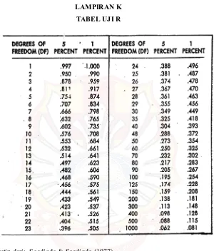
LAMPIRAN K TABEL UJI R
LAMPIRAN L
HASIL UJI ANAVA KEKERASAN TABLET DENGAN DESIGN EXPERT
Response 1 Kekerasan ANOVA for selected factorial model
Analysis of variance table [Partial sum of squares - Type III] Sum of Mean F p-value Source Squares df Square Value Prob >F
Model 7.30 3 2.43 88.43 < 0.0001 significant
The Model F-value of 88.43 implies the model is significant. There is only
a 0.01% chance that a "Model F-Value" this large could occur due to noise.
Values of "Prob > F" less than 0.0500 indicate model terms are significant.
In this case A, B, AB are significant model terms.
Values greater than 0.1000 indicate the model terms are not significant. If there are many insignificant model terms (not counting those required to support hierarchy),
model reduction may improve your model.
Std. Dev. 0.17 R-Squared 0.9707 Mean 6.22 Adj R-Squared 0.9597 C.V. % 2.67 Pred R-Squared 0.9341 PRESS 0.50 Adeq Precision 21.823
The "Pred R-Squared" of 0.9341 is in reasonable agreement with the "Adj R-Squared" of 0.9597.
"Adeq Precision" measures the signal to noise ratio. A ratio greater than 4 is desirable. Your
navigate the design space.
Final Equation in Terms of Coded Factors:
Kekerasan =
+6.22
+0.54 * A
-0.51 * B
+0.25 * A * B
Final Equation in Terms of Actual Factors:
Kekerasan =
+6.68000
+6.30556E-003 * Avicel
-0.41667 * SSG
+4.13889E-003 * Avicel * SSG
The Diagnostics Case Statistics Report has been moved to the Diagnostics Node.
In the Diagnostics Node, Select Case Statistics from the View Menu.
Proceed to Diagnostic Plots (the next icon in progression). Be sure to look at the:
1) Normal probability plot of the studentized residuals to check for normality of residuals.
constant error.
3) Externally Studentized Residuals to look for outliers, i.e., influential values.
4) Box-Cox plot for power transformations.
LAMPIRAN M
HASIL UJI ANAVA KERAPUHAN TABLET DENGAN DESIGN EXPERT
Response 2 Kerapuhan ANOVA for selected factorial model
Analysis of variance table [Partial sum of squares - Type III] Sum of Mean F p-value
The Model F-value of 617.25 implies the model is significant. There is only
a 0.01% chance that a "Model F-Value" this large could occur due to noise.
Values of "Prob > F" less than 0.0500 indicate model terms are significant.
In this case A, B, AB are significant model terms.
Values greater than 0.1000 indicate the model terms are not significant. If there are many insignificant model terms (not counting those required to support hierarchy),
model reduction may improve your model.
Std. Dev. 0.015 R-Squared 0.9957 Mean 0.27 Adj R-Squared 0.9941 C.V. % 5.48 Pred R-Squared 0.9903 PRESS 3.926E-003 Adeq Precision 56.278
The "Pred R-Squared" of 0.9903 is in reasonable agreement with the "Adj R-Squared" of 0.9941.
"Adeq Precision" measures the signal to noise ratio. A ratio greater than 4 is desirable. Your
navigate the design space.
Coefficient Standard 95% CI 95% CI Factor Estimate df Error Low High Intercept 0.27 1 4.263E-003 0.26 0.28
A-Avicel -0.15 1 4.263E-003 -0.16 -0.14 B-SSG 0.086 1 4.263E-003 0.077 0.096 AB -0.051 1 4.263E-003 -0.061 -0.041
Final Equation in Terms of Coded Factors:
Kerapuhan =
+0.27
-0.15 * A
+0.086 * B
-0.051 * A * B
Final Equation in Terms of Actual Factors:
Kerapuhan =
+0.32921
-3.40000E-003 * Avicel
+0.080094 * SSG
-8.54583E-004 * Avicel * SSG
The Diagnostics Case Statistics Report has been moved to the Diagnostics Node.
In the Diagnostics Node, Select Case Statistics from the View Menu.
Proceed to Diagnostic Plots (the next icon in progression). Be sure to look at the:
1) Normal probability plot of the studentized residuals to check for normality of residuals.
2) Studentized residuals versus predicted values to check for constant error.
values.
4) Box-Cox plot for power transformations.
LAMPIRAN N
HASIL UJI ANAVA WAKTU HANCUR TABLET DENGAN DESIGN EXPERT
Response 3 Waktu hancur ANOVA for selected factorial model
Analysis of variance table [Partial sum of squares - Type III] Sum of Mean F p-value
The Model F-value of 537.77 implies the model is significant. There is only
a 0.01% chance that a "Model F-Value" this large could occur due to noise.
Values of "Prob > F" less than 0.0500 indicate model terms are significant.
In this case A, B, AB are significant model terms.
Values greater than 0.1000 indicate the model terms are not significant. If there are many insignificant model terms (not counting those required to support hierarchy),
model reduction may improve your model.
Std. Dev. 0.12 R-Squared 0.9951 Mean 3.09 Adj R-Squared 0.9932 C.V. % 3.91 Pred R-Squared 0.9889 PRESS 0.26 Adeq Precision 54.502
The "Pred R-Squared" of 0.9889 is in reasonable agreement with the "Adj R-Squared" of 0.9932.
"Adeq Precision" measures the signal to noise ratio. A ratio greater than 4 is desirable. Your
navigate the design space.
Coefficient Standard 95% CI 95% CI Factor Estimate df Error Low High Intercept 3.09 1 0.035 3.01 3.17 A-Avicel 0.70 1 0.035 0.62 0.78 B-SSG -1.20 1 0.035 -1.28 1.12 AB -0.17 1 0.035 -0.26 -0.095
Final Equation in Terms of Coded Factors:
Waktu hancur =
+3.09
+0.70 * A
-1.20 * B
-0.17 * A * B
Final Equation in Terms of Actual Factors:
Waktu hancur =
+2.11667
+0.049583 * Avicel
-0.22500 * SSG
-2.91667E-003 * Avicel * SSG
The Diagnostics Case Statistics Report has been moved to the Diagnostics Node.
In the Diagnostics Node, Select Case Statistics from the View Menu.
Proceed to Diagnostic Plots (the next icon in progression). Be sure to look at the:
1) Normal probability plot of the studentized residuals to check for normality of residuals.
2) Studentized residuals versus predicted values to check for constant error.
values.
4) Box-Cox plot for power transformations.
LAMPIRAN O
HASIL UJI ANAVA PERSEN OBAT TERLARUT DALAM T = 15 MENIT DENGAN DESIGN EXPERT
Response 4. Disolusi
ANOVA for selected factorial model
Analysis of variance table [Partial sum of squares - Type III] Sum of Mean F p-value
Source Squares df Square Value Prob > F
Model 191.28 3 63.76 329.83 < 0.0001significant
The Model F-value of 329.83 implies the model is significant. There is only
a 0.01% chance that a "Model F-Value" this large could occur due to noise.
Values of "Prob > F" less than 0.0500 indicate model terms are significant.
In this case A, B, AB are significant model terms.
Values greater than 0.1000 indicate the model terms are not significant. If there are many insignificant model terms (not counting those required to support hierarchy),
model reduction may improve your model.
Std. Dev. 0.44 R-Squared 0.9920 Mean88.66 Adj R-Squared 0.9890 C.V. % 0.50 Pred R-Squared 0.9820 PRESS 3.48 Adeq Precision 41.761
The "Pred R-Squared" of 0.9820 is in reasonable agreement with the "Adj R-Squared" of 0.9890.
ratio of 41.761 indicates an adequate signal. This model can be used to navigate the design space.
Coefficient Standard 95% CI 95% CI
Factor Estimate df Error Low High VIF Intercept 88.66 1 0.13 88.37 88.95
A-Avicel -1.99 1 0.13 -2.29 -1.70 1.00 B-SSG 3.31 1 0.13 3.01 3.60 1.00 AB1.02 1 0.13 0.72 1.31 1.00
Final Equation in Terms of Coded Factors:
Final Equation in Terms of Actual Factors:
The Diagnostics Case Statistics Report has been moved to the Diagnostics Node.
In the Diagnostics Node, Select Case Statistics from the View Menu.
Proceed to Diagnostic Plots (the next icon in progression). Be sure to look at the:
1) Normal probability plot of the studentized residuals to check for normality of residuals.
2) Studentized residuals versus predicted values to check for constant error.
3) Externally Studentized Residuals to look for outliers, i.e., influential values.
LAMPIRAN P
UJI F KURVA BAKU PENETAPAN KADAR Uji Kesamaan Regresi (Aquadest)
REPLIKASI 1
KONSENTRASI ABSORBANSI X2 Y2 XY
32.192 1.141 1036.3249 1.3019 36.7311
48.288 1.303 2331.7309 1.6978 62.9193
64.384 1.432 4145.2995 2.0506 92.1979
80.48 1.603 6477.0304 2.5696 129.0094
96.576 1.711 9326.9238 2.9275 165.2415
23317.3094 10.5474 486.0992
REPLIKASI 2
KONSENTRASI ABSORBANSI X2 Y2 XY
32.064 0.957 1028.1001 0.9158 30.6852
48.096 1.103 2313.2252 1.2166 53.0499
64.128 1.232 4112.4004 1.5178 79.0057
80.16 1.423 6425.6256 2.0249 114.0677
96.192 1.551 9252.9009 2.4056 149.1938
23132.2522 8.0808 426.0023
REPLIKASI 3
KONSENTRASI ABSORBANSI X2 Y2 XY
32.128 1.141 1032.2084 1.3019 36.6580
48.192 1.353 2322.4689 1.8306 65.2038
64.256 1.531 4128.8335 2.3440 98.3759
80.32 1.723 6451.3024 2.9687 138.3914
96.384 1.871 9289.8755 3.5006 180.3345
S X2 SXY S Y2 N SSi RDF Regresi I 23317.3094 486.0992 10.5474 5 10.5266 4 Regresi II 23132.2522 426.0023 8.0808 5 8.0624 4 Regresi III 23224.6886 518.9636 11.9458 5 11.9235 4
69674.2502 1431.0651 30.5741 30.5125 SSc = 30.55353763
LAMPIRAN Q
UJI F KURVA BAKU DISOLUSI Uji Kesamaan Regresi (Dapar fosfat pH 6,8)
REPLIKASI 1
KONSENTRASI ABSORBANSI X2 Y2 XY
32.192 1.141 1036.3249 1.3019 36.7311
48.288 1.303 2331.7309 1.6978 62.9193
64.384 1.432 4145.2995 2.0506 92.1979
80.48 1.603 6477.0304 2.5696 129.0094
96.576 1.711 9326.9238 2.9275 165.2415
REPLIKASI 2
KONSENTRASI ABSORBANSI X2 Y2 XY
32.064 0.957 1028.1001 0.9158 30.6852
48.096 1.103 2313.2252 1.2166 53.0499
64.128 1.232 4112.4004 1.5178 79.0057
80.16 1.423 6425.6256 2.0249 114.0677
96.192 1.551 9252.9009 2.4056 149.1938
REPLIKASI 3
KONSENTRASI ABSORBANSI X2 Y2 XY
32.128 1.141 1032.2084 1.3019 36.6580
48.192 1.353 2322.4689 1.8306 65.2038
64.256 1.531 4128.8335 2.3440 98.3759
80.32 1.723 6451.3024 2.9687 138.3914
96.384 1.871 9289.8755 3.5006 180.3345
6 X2 6XY 6 Y2 N SSi RDF
Regresi I 5 10.5266 4
Regresi II 5 8.0624 4
Regresi III 5 11.9235 4
69674.2502 1431.0651 30.5741 30.5125
SSc= 30.55353763
F= 0.008075857 < Ftabel 3,89