Vol. 44 (2001) 55–69
Agency costs, asset specificity, and the capital
structure of the firm
Jon Vilasuso
a,∗, Alanson Minkler
baDepartment of Economics, West Virginia University, Box 6025, Morgantown, WV 26506-6025, USA bDepartment of Economics, University of Connecticut, Box U-63, Storrs, CT 06269-1063, USA
Received 4 February 1998; received in revised form 9 May 2000; accepted 2 June 2000
Abstract
We develop a dynamic model that incorporates the insights of both the agency cost and asset specificity literature about corporate finance. In general, we find that neither can be ignored, and that the optimal capital structure minimizes agency cost and asset specificity considerations. A key finding is that the conditions most favorable for reducing transaction costs due to asset specificity are the same as those for reducing the agency costs of debt. Empirically, we find that agency costs and asset specificity are significant determinants of a firm’s capital structure in the transportation equipment and the printing and publishing industries. © 2001 Elsevier Science B.V. All rights reserved.
JEL classification: G32
Keywords: Capital structure; Financing policy
1. Introduction
In a seminal paper, Modigliani and Miller (1958) demonstrated that the value of a firm and its capital costs are independent of its capital structure, thereby dismissing the notion of an optimal capital structure. While challenged almost immediately, it is generally accepted today that the Modigliani–Miller results are attributed to the existence of perfect capital markets.1 Imperfect capital markets, in contrast, offer an explanation for why actual firms
∗Corresponding author.
1Modigliani and Miller (1958) do show that the value of a firm is affected if firms can borrow at a lower cost than can investors, thereby eliminating perfect capital markets. Additionally, tax considerations (Modigliani and Miller, 1963; DeAngelo and Masulis, 1980), brokerage costs (Baumol and Malkiel, 1967), segmented markets (Stiglitz, 1972), and bankruptcy costs (Scott, 1976) break the invariance results of Modigliani and Miller (1958). Recent surveys and discussions include Masulis (1988), Miller (1988), Ross (1988), Stiglitz (1988), Bhattacharya (1988), and Modigliani (1988).
deliberate not only about different potential investment projects but also over the way in which projects are financed. In this paper, we develop a model of the capital structure of the firm in an imperfect capital market setting due to agency costs and asset specificity considerations stressed by transaction cost economics.2 In general, we find that both agency costs and asset specificity influence the firm’s capital structure, and focusing on just one or the other may lead to erroneous predictions about the firm’s optimal capital structure.
The effects of agency costs on the capital structure are examined by Jensen and Meckling (1976). Jensen and Meckling explain that as an owner/manager dilutes his ownership by issuing outside equity, he may be induced to pursue greater non-pecuniary benefits because he can share the cost with the new owners. New equity owners are aware of this agency problem, and consequently reduce the price they are willing to pay for the new shares, thereby increasing the cost of new equity.3The argument continues to cover the issuance of debt claims. If the firm issues new debt, then bondholders will be cautious if they believe that they are vulnerable to excessive risk taking by equity owners who benefit disproportionately
if the firm is highly leveraged. Thus, the cost of debt is increasing in leverage. The optimal
capital structure then minimizes the sum of the agency costs of debt and equity.
Transaction cost economics focuses on the technological factors of production and the different governance methods implied (Williamson, 1988). If an investment project requires assets that are highly specific to the project and have little value otherwise, then bondholders are vulnerable to expropriation by the managers of the firm because bondholders are not entitled to control. Equity, in contrast, involves control and a firm’s board of directors can be seen as an attempt to attenuate the opportunities of the managers from expropriating quasi-rents. Thus, if the firm’s investment project entails highly specific assets then they are financed with equity, while debt finance is used if assets are more generic and can be easily redeployed.4
The purpose of this paper is to integrate the insights of the agency cost and asset specificity literature into a single framework. To the agency cost literature we add the important notion of the hazard of asset specificity. To the asset specificity literature we add the agency costs confronted by bondholders due to equity holder behavior. A key insight is that for highly specific assets, equity reduces transaction costs by limiting opportunistic behavior, but over time additional equity also offers bondholders greater protection from excessive risk taking which reduces the agency costs of debt. To see this result, consider the following example: suppose that an investment project involves highly specific assets and initially equity finance is less expensive than is debt finance due to asset specificity considerations. In the first period,
2Imperfect capital markets may also be traced to asymmetric information (Ross, 1977; Myers and Majluf, 1984; Grossman and Hart, 1982), the nature of product markets (Brander and Lewis, 1986), and corporate control considerations (Harris and Raviv, 1988; Stutz, 1988). See Harris and Raviv (1991) for a review of this literature. 3The owner/manager can improve his own welfare by allowing new shareholders to monitor him, thereby controlling his non-pecuniary consumption. Monitoring, however, is likely to be costly. The conflict between the owner/manager and outside shareholders can also be reduced by issuing debt. Debt mitigates this conflict because it reduces free cash flow (Jensen, 1986), and if bankruptcy is costly for the owner/manager, then debt can provide an incentive to consume fewer perquisites (Grossman and Hart, 1982).
equity is used as suggested by the asset specificity literature. But as the capital structure of the firm relies more heavily on equity finance, agency cost considerations suggest that the cost of equity rises but the cost of debt finance falls as bondholders become less vulnerable to excessive risk taking by shareholders. So while reduced leverage provides enhanced internal control, it also provides the most safeguards for bondholders because they have first claim. The remainder of the paper is organized as follows. In Section 2 we develop a dynamic capital structure model where an ongoing investment project is financed with external funds. Section 3 explores the properties of the model. We find that the firm uses both debt and equity, and the optimal capital structure of the firm minimizes the sum of agency costs and costs aris-ing from asset specificity. In addition, we demonstrate that special cases do exist where either agency cost or asset specificity factors dominate. In Section 4, we empirically test the predic-tions of the model and find that both agency costs and asset specificity are important deter-minants of the capital structure of the firm. The final section presents concluding comments.
2. The capital structure of the firm
In this section, we present a dynamic model of the firm’s capital structure where the cost of project finance is affected by both agency costs and the degree of asset specificity exhibited by the investment project. The model examines an ongoing project that is financed with external funds by issuing debt, equity, or some combination.
The capital structure of the firm at time t is represented by the debt–equity mix:
θ (t )=[D0+D(t )]−[E0+E(t )] (1)
where D0and E0are the initial (exogenous) stocks of debt and equity, respectively. The
stock of debt finance is D(t), and E(t) represents the stock of equity finance. The debt–equity mix evolves according to
˙
θ (t )=d(t )−e(t ) (2)
where d(t) is the flow of debt finance and e(t) is the flow of equity finance. The termθ(t) can be expressed as the ratio of total debt to equity; the results to follow would be unchanged. We choose to use the debt–equity mix in an effort to simplify the analysis.
The amount of financial capital needed for the investment project, I, is assumed exoge-nous. We rule out recapitalization which implies that
e(t )+d(t )=I. (3)
The assumption of no recapitalization ensures that both e(t) and d(t) are bound by the closed interval [0, I]. Solving (3) for d(t) and substituting this expression into (2) allows the change in the debt–equity mix to be written in terms of new equity finance:
˙
θ (t )=I−2e(t ). (4)
The investment project is characterized by a degree of asset specificity, k, that is tech-nologically determined such thatk ∈[0,k¯] andk >¯ 0 is finite. A high value of k implies that the investment project involves assets that are difficult to redeploy and have little value outside the current application. Thus, a high value of k implies that the investment project exhibits a high degree of asset specificity.
The agency costs of obtaining external capital trace to incentive-alignment issues in an incomplete information setting. The effects of agency costs on the cost of capital detailed here draws on the work of Jensen and Meckling (1976). Consider an investment project where x represents productive assets involved with the project. The level of profit associated with the project is given byπ(x) and is a random variable with distribution function G defined over the closed interval [π
¯,π¯] whereπ¯ <0 andπ >¯ 0. The mean isπˆ and the variance isσ2. As in Jensen and Meckling, we assume that x yields positive marginal utility to the owner/manager. Let x∗represent assets devoted to production, in which case,x−x∗denotes the owner/manager’s non-pecuniary consumption. The value of non-pecuniary consumption is then given byF =π(x)−π(x∗)≥0.5The (expected) value of the firm, V∗, is determined as the discounted value of profits whereV∗= ¯V −F such thatV¯ is defined forF =0.
Should the owner/manager issue outside equity claims, a rational investor realizes that there is an incentive for the owner/manager to increase his non-pecuniary consumption because the owner/manager does not bear the full cost of doing so. As a result, F increases relative to the case where the owner/manager has full equity in the firm. Consequently, the price that an investor is willing to pay for equity shares declines. Or put differently, the cost of equity can be interpreted as the discount factor used to compute V∗and the cost of equity increases as the owner/manager relinquishes a larger ownership stake. Ifce(k, θ (t ))
represents the cost of outside equity, the agency costs of equity hold that
∂ce(k, θ (t )) ∂θ (t ) =c
e
θ(k, θ (t )) <0. (5)
That is, an increase in equity finance (relative to debt finance) reduces leverage and raises the cost of equity.
The agency costs of debt stem from the owner/manager’s incentive to reallocate wealth from bondholders to himself (and by proxy, other outside shareholders). Jensen and Meck-ling (1976) explain that in the case of debt finance, the owner/manger will be induced to pursue high risk-high return projects. Consider, for example, a mean-preserving spreadG¯
(i.e. with meanπˆ and varianceσ¯2> σ2). Also, considerπ′such thatπ′>πˆ. It follows that
(1− ¯G(π′)) > (1−G(π′)), suggesting that the probability of a high payout is greater for ¯
G; but it also follows that the probability of a low payout is greater asG(¯ πˆ−(π′− ˆπ )) > G(πˆ −(π′− ˆπ )). As the residual claimant, the (risk neutral) owner/manager prefersG¯
because shareholders will capture the benefits of success but do not bear the full cost of failure. Ifcdθ(k, θ (t ))represents the cost of debt, then
∂cd(k, θ (t )) ∂θ (t ) =c
d
θ(k, θ (t )) >0 (6)
which states that greater leverage leads to excessive risk taking and rational investors demand a higher return on debt.6
The effects of asset specificity on the cost of capital trace to an ex post occurrence of bankruptcy, in which case the assets associated with the investment project are liquidated. The ex ante probability of bankruptcy, on the other hand, is driven by agency cost consider-ations.7 Let s(k) denote the salvage value of the physical assets in the event of bankruptcy wheres(k)≤ I. Also, suppose that bankruptcy takes place ifπ ≤πbwhich occurs with probability G(πb). Following the definition of asset specificity advanced by Williamson (1988),∂s(k)/∂k < 0. An increase in k produces a decline in s(k), thereby reducing the payout to claim holders in the event of bankruptcy. Thus, the cost of equity and debt are both increasing in k. The cost of debt, however, rises faster. In the case of debt finance, the owner/manager is more likely to pursue the riskier project characterized byG¯ such that
¯
G(πb) > G(πb). Thus, the likelihood of bankruptcy is greater, and as a result8
∂cd(k, θ (t )) ∂k >
∂ce(k, θ (t ))
∂k >0 (7)
whereckd(k, θ (t ))andcek(k, θ (t ))represent the partial derivatives in (7). If debt finance involves a lower setup cost, then (7) implies that there exists a critical value of asset speci-ficity, saykˆ, where debt is used for all projectsk <kˆand equity finance is less expensive ifk >kˆ.9
The total cost of financing the investment project is
C(t )=[e(t )ce(k, θ (t ))]+[(I−e(t ))cd(k, θ (t ))] (8)
where the first bracketed term is the total cost of equity finance and the second bracketed term is the total cost of debt finance. It is instructive to consider how a change in the amount of equity finance obtained affects the total cost of project finance:
∂C(t ) ∂e(t ) =[c
e(k, θ (t ))−cd(k, θ (t ))]−2[ece
θ(k, θ (t ))+(I−e)cθd(k, θ (t ))]. (9)
6Expression (5) and (6) are consistent with the agency costs of debt and equity represented in Fig. 5 of Jensen and Meckling (1976) (p. 344). In addition, total agency costs are convex inθwhich requires thatcθ θd (·)+ceθ θ(·) >0
wherecjθ θ(·)≡∂2cj(·)/∂θ2.
7The descriptions of the influence of agency costs and asset specificity are consistent with the work of Williamson (1988). Williamson writes that agency cost theory takes an ‘ex ante incentive-alignment’ point of view while asset specificity considerations are more concerned with ‘crafting ex post governance structures’ (p. 570).
8Williamson (1988) offers a governance structure explanation. Debt is a rule-based governance structure and a ‘rule-governed regime will sometimes force liquidation or otherwise cause the firm to compromise value-enhancing decisions’ than does a more flexible or adaptive regime such as equity (p. 580). In the notation developed above, Williamson’s argument implies thatπbis greater under a debt regime than is the case for equity. This explanation is also consistent with expression (7), given setup costs.
The first bracketed term captures the influence of asset specificity. For example, once the value of k is given, the first bracketed term measures the direct cost (ifk <kˆ) or benefit (if
k >kˆ) of equity finance. Note that the influence of asset specificity measures the difference in the cost functions without regard to the capital structure of the firm. In contrast, the second bracketed term focuses on the consequences of altering the firm’s capital structure. That is, the second bracketed term represents the agency costs of increasing equity in the firm’s capital structure, which ultimately affects the cost of capital, but is silent in regards to the characteristics of the investment project.
The firm’s planning problem is then to minimize the cost of external funds (8) subject to the constraint that the project is fully financed (3) over the investment horizon [0,T]. Formally, the firm selects the optimal control, e∗, that solves
Minimize Z T
t=0
[ece(k, θ )+(I−e)cd(k, θ )] dt,
Subject toθ˙=I−2eande∈[0, I]. (10)
The time notation is omitted where understood. The Hamiltonian is
H (θ, e, λ)=[ece(k, θ )+(I−e)cd(k, θ )]+λ(I−2e] (11)
whereλis the costate variable which measures the shadow value of leverage. The Hamil-tonian represent the total cost of choosing e: the sum of current costs, as represented by the bracketed term and the value of altering leverage represented by the second term. Thus, the Hamiltonian encompasses both the immediate and future effects of the firm’s financing decision.
The maximum principle conditions are
Max
e −H (θ, e, λ)for allt∈[0, T] (12)
˙
θ=Hλ(θ, e, λ)=I −2e (13)
˙
λ= −Hθ(θ, e, λ)= −[eceθ(k, θ )+(I−e)cθd(k, θ )]. (14)
Condition (12) implies that the firm minimizes the total cost by choosing the optimal value of e that balances current and future costs. This condition recognizes that the current choice of equity finance affects the firm’s leverage, and hence future capital costs. Condition (13) is the equation of motion for the state variable and merely specifies how the current financing policy affects leverage. Condition (14) describes the equation of motion of the costate variable and represents the marginal contribution of leverage to the cost of both debt and equity. That is, condition (14) equates the rate of change of the shadow value of leverage and the marginal contribution of leverage to current capital costs, or put differently, this condition captures the agency costs of altering the firm’s capital structure.
Because H(·) is linear in e ande∈[0, I], condition (12) does not require that He(·)=0.
Instead, the sign of
is evaluated. The optimal control is then set according to
which compares the average difference between the cost functions and the shadow value of the debt–equity mix.
The optimal control balances both agency cost and asset specificity considerations. The term (ce(·)−cd(·))/2 in condition (16) examines the difference between the cost of equity and the cost of debt for a given value of asset specificity. But because the investment project is ongoing, the firm’s capital structure also evolves over time. As a result, the agency costs of debt and equity are altered as represented in (14). Consequently, the contribution of agency costs is described by the termλincluded in expression (16).
The optimal debt–equity mix, as determined by (16), depends on the capital structure of the firm as well as characteristics of the investment project. That is, the characteristics of the project reflect the degree of asset specificity, while the capital structure defines the importance of agency costs.
3. Dynamic properties of the model
We now investigate the firm’s optimal financing strategy in the following propositions. Formal proofs of the propositions are given in the Appendix A.
Proposition 1. Over a long investment horizon, the optimal capital structure, θ∗, uses both debt and equity finance to minimize the sum of agency cost and asset specificity considerations.
Proposition 2. Over a long investment horizon, the agency costs of debt and equity
em-bodied inθensure that the capital structure of the firm converges to its optimal value for a given value of k.
As in Proposition 1, consider a firm that finances a highly asset specific project such that the cost of equity is strictly less than the cost of debt. Although initially the firm pursues a pure equity finance policy, agency costs are still operative. As the firm becomes less levered, the agency costs of debt decline while the agency costs of equity rise until the cost of debt rivals that of equity. Thus, agency costs, as embodied in the path ofθensure that the firm switches to debt finance over a long investment horizon and the firm’s capital converges to its optimal value for a given value of asset specificity.
Proposition 3 focuses on the influence of asset specificity on the optimal capital structure of the firm.
Proposition 3. Over a long investment horizon, the optimal capital structureθ∗uses more equity finance as the degree of asset specificity increases, all else equal.
Proposition 3 notes that although the optimal financing strategy uses both debt and equity to minimize the sum of agency and asset specificity considerations, an increase in asset specificity favors a less levered capital structure. For example, consider two firms that differ only in terms of the type of investment project that is financed. Also, assume that initially the cost of debt exceeds the cost of equity for each project. The difference between the costs of debt and equity, however, is greater for the project that exhibits the higher degree of asset specificity. In the first period, equity finance is cost minimizing for each project. As leverage declines, the cost of equity rises and the cost of debt falls, and eventually agency costs favor debt and each firm switches as described in Proposition 2. But the point at which each firm switches to debt finance is not the same. The firm that finances the project exhibiting the higher degree of asset specificity switches to debt strictly later than the other firm. Put differently, agency cost considerations take longer to ‘catch up’ as the degree of asset specificity increases, and as a result, the firm relies more heavily on equity finance if assets are more difficult to redeploy.
The next two propositions describe the solutions to the model when only agency costs or the degree of asset specificity need to be considered in the firm’s financing policy. Asset specificity considerations dominate, and hence all equity finance is optimal for a highly asset specific project under the following conditions.10
Proposition 4. Only the degree of asset specificity needs to be considered if (a) the
in-vestment horizon, T, approaches zero; (b) total project finance needs, I, are slight, and (c)
θ0=D0−E0is positively related to k.
Essentially, the restrictions described above force the dynamic model to collapse to a static model where agency cost considerations can be ignored because new financing needs do not significantly alter the firm’s existing capital structure. Under these restrictions, the
model reduces to the transaction cost economics approach where projectsk >kˆuse equity while projectsk <kˆare debt financed.
The agency cost approach is a special case if a restriction is placed on the cost functions.
Proposition 5. Ifckd(·)=cek(·), then the agency cost approach is optimal andθ∗is inde-pendent of k for all t.
Proposition 5 shows that if the cost of debt and equity vary by the same amount for a parametric change in the degree of asset specificity, then the optimal capital structure of the firm does not depend on asset specificity. Intuitively, this restriction on the cost functions suggests that the influence of asset specificity is the same for all investment projects. A change in the degree of asset specificity produces the same discrepancy between the costs of debt and equity, and in this case, agency costs ‘catch up’ at the same point for all projects. The end result is that the firm pursues a financing strategy, and hence an optimal capital structure, that is invariant to asset specificity.
In general neither agency costs nor asset specificity can be ignored as determinants of the optimal capital structure of the firm. Still, special cases do exist in which only one or the other is determinant. These special cases, however, follow from placing restrictions on either the dynamics of the model or on the costs of obtaining external funds.
4. The empirical model
In this section we empirically test the predictions of the model that links both agency costs and asset specificity to the capital structure of the firm. The influence of asset specificity is included as a determinant of the firm’s optimal capital structure (Proposition 3), while agency cost considerations ensure that the firm’s capital structure converges to its optimal value (Proposition 2).
The agency costs of external finance, as embodied inθ, ensure thatθ converges to its optimal value. An account of the dynamic adjustment process for firm i at time t is
(θi,t −θi,t∗−1)=α1(θi,t−1−θi,t∗−1) (17)
for a given value ofθi,t∗−1. The effects of agency costs are represented by the restriction that|α1| <1 which stipulates thatθ → θ∗ ast → ∞. Turning to the influence of asset specificity, the optimal capital structure is inversely related to the degree of asset specificity of the investment project. A linear account of this relation is given by
θi,t∗−1=a0+a1ki,t−1. (18)
The theoretical model then predicts thata1 < 0, suggested that a higher degree of asset
specificity favors a lower value of leverage. Combining expressions (17) and (18) yields the empirical model:
θi,t =a0(1−α1)+α1θi,t−1+a1(1−α1)ki,t−1. (19)
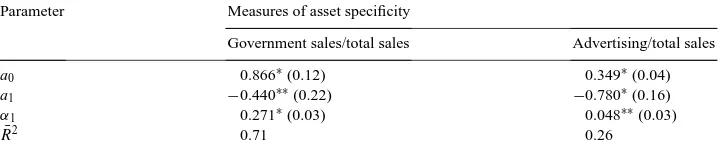
Table 1
Parameter estimatesa
Parameter Measures of asset specificity
Government sales/total sales Advertising/total sales
a0 0.866∗(0.12) 0.349∗(0.04)
a1 −0.440∗∗(0.22) −0.780∗(0.16)
α1 0.271∗(0.03) 0.048∗∗(0.03)
¯
R2 0.71 0.26
aParameter estimates are determined using nonlinear least squares. Standard errors are in parentheses and are adjusted for heteroskedasticity.
∗Denotes statistical significance at the 1-percent level. ∗∗Denotes the 5-percent level.
Assuming that the determinants of agency costs are similar across firms within an industry, the empirical model holds that the firm’s capital structure is a function of its lagged capital structure and the degree of asset specificity.11 Agency costs nevertheless play a role in determining the actual capital structure at a point in time. Because the degree of asset specificity is not directly observable, a proxy must be constructed. Alternative proxies are considered in turn.
4.1. Government procurement
The first measure of asset specificity considered is the ratio of sales to the government to total sales. Crocker and Reynolds (1993) (p. 129) explain that government procurement, by its very nature, ‘involves substantial recurring investment in relationship-specific assets,’ especially in the case of defense contracting.12 As such, assets dedicated to government procurement represent highly asset specific investment, and the share of total sales to the government13 is used as a proxy for the degree of asset specificity.14
The sample consists of 28 publicly held firms whose primary industrial classification is transportation equipment, which includes aircraft, defense, and space vehicles and compo-nents. A total of 138 observations are available. Parameter estimates are collected in the first column of Table 1. Estimates of the empirical model are consistent with the predictions of the theoretical model. The influence of asset specificity, captured by a1, is negative as
expected and is statistically significant at the 5-percent level, suggesting an inverse relation between leverage and asset specificity. The influence of agency costs, captured byα1, holds
that the capital structure of the firm does indeed converge to its optimal level.
11We follow the advice of Masten (1984) and focus on a specific industry as the ‘level of detail’ needed to control for cross-industry effects can impede empirical work.
12Crocker and Reynolds (1993) find that in the case of Air Force engine procurement, the degree of contract completeness balances ex ante contracting costs and ex post opportunism.
4.2. Advertising expenditure
The next proxy for asset specificity investigated is the ratio of advertising expenditure to total sales for a sample of firms whose primary SIC is printing and publishing. In an influential work, Sutton (1991) argues that endogenous sunk costs such as advertising is a firm-level strategic decision so as to affect a consumer’s willingness to pay for the firm’s product.15 Because an endogenous sunk cost can not be recovered (it has no salvage value), advertising expenditure has little value outside of its current transaction, and as such exhibits a high degree of asset specificity.16 The printing and publishing industry exhibits a high level of advertising intensity,17 and the advertising/sales ratio is used to measure the degree of asset specificity in this industry.
Parameter estimates are listed in the second column of Table 1. The sample consists of 37 firms that yield 117 observations. Parameter estimates support the predictions of the theoretical model. The parameter a1is negative as expected and is statistically significant
at the 1-percent level. Agency cost considerations are also supported by the data as the null hypothesis|α1|<1 can not be rejected at conventional significance levels.
5. Conclusion
In this paper, we present a dynamic model of a firm’s financing policy where debt, equity, or some combination is used to finance an ongoing investment project. The model incorporates both agency cost and asset specificity considerations. The cost of external funds depends on both the characteristics of the assets involved in the project — asset specificity — and the changing incentive structure faced by debt and shareholders — agency costs.
The model demonstrates that both agency costs and asset specificity influence the firm’s financing policy, and focusing on just one or the other may not accurately describe the optimal capital structure of the firm. The main finding is that although equity finance reduces transaction costs when assets are highly specific, equity finance also offers bondholders greater protection from excessive risk taking which reduces the agency costs of debt. As a result, the optimal capital structure of the firm uses both debt and equity finance to minimize the sum of agency cost and asset specificity considerations.
We find that both agency costs and asset specificity are significant determinants of the firm’s capital structure in both the transportation equipment and the printing and publishing industries. In future work we plan to expand the number of industries under consideration and explore alternative measures of asset specificity.
15An exogenous sunk cost is outside the control of an individual firm and is better viewed as an industry charac-teristic. An example offered by Sutton (1991) is the cost of developing a minimum efficient scale plant.
16Although advertising expenditure has been viewed as a means of restricting competition and new entry, Szenberg and Lee (1995) find that the minimum efficient scale of production in publishing is low, and advertising can not substantially reduce competition nor obstruct new entry.
Acknowledgements
We thank Richard Day (Editor), Mark Frascatore, Thomas Miceli, Stephen Miller, and two anonymous referees for helpful comments on an earlier draft of this paper.
Appendix A
A.1. Proof of Proposition 1
For notional purposes, defineJ (k, θ ) ≡ (ce(·)−cd(·))/2 wherejθ(k, θ ) = (ceθ(·)−
cdθ(·))/2 < 0 from (5) and (6). The strategy employed is to consider a set of initial conditions that most favor the influence of asset specificity, and then demonstrate that a financing plan that includes both debt and equity is less costly. Consider the initial conditions such that J (k, θ ) < 0 at t = 0 which suggests that the project exhibits a high degree of asset specificity. Also, let I = 1 so that one unit of external finance is secured over the investment horizon. Suppose that contrary to Proposition 1, the firm finances the project solely with equity consistent with asset specificity considerations stressed in the transaction cost economics literature. For the horizon [0,T], total invest-ment is just T and the resultant debt–equity mix is θ0 − T. Total financing costs
are Z θ0
θ0−T
ce(k, θ )dθ = Z θ0−t∗
θ0−T
ce(k, θ )dθ+ Z θ0
θ0−t∗
ce(k, θ )dθ (A.1)
for somet∗< T. This transaction cost economic approach, however, is not cost minimizing. Ife∗=1, thenθ <˙ 0 from (13). Becauseθis declining, the cost of debt falls and the cost of equity rises. Consequently, J(·) is increasing due to agency cost considerations. For a sufficiently long investment horizon, there exists somet∗< T such thatJ (k, θ0−t∗)≈
0. Thus, at time t∗ the firm switches from equity finance to debt finance according to (16). For finite T, there exists a set of pointst∗+ifor positive i such that total costs are approximately
Z θ0
θ0−t∗
ce(k, θ )dθ+(T −t∗)ce(k, θ (t∗)) (A.2)
force(k, θ (t∗))≈cd(k, θ (t∗)). This solution uses equity up to time t∗and then oscillates between debt and equity finance over the remainder of the investment horizon. Because
ce(k, θ (t∗)) < ce(k, θ (T ))for allt∗ < T, total costs given by (A.2) are strictly less than total costs given by (A.1). Therefore, E(t),D(t ) > 0. ForJ (k, θ ) ≥0 at timet =0, the proof is similar.
A.2. Proof of Proposition 2
Consider a highly asset specific project such thatJ (k, θ ) <0 at timet = 0. Also, let
Put differently, agency costs ensure the existence of t∗, which in turn defines the optimal debt–equity mixθ∗=θ∗(k). Thus, agency cost considerations ensure thatθconverges toθ∗. DefineA(k, θ ) ≡ [cd(·)−ce(·)] which measures the difference between the cost of debt and the cost of equity. Because the project exhibits a high degree of asset specificity,
A(k, θ ) >0 at timet =0. Agency costs influence the cost functions such that
∂A(k, θ )
from expressions (5) and (6). At timet = 0, equity finance is cost minimizing. But as leverage falls,θ <˙ 0 and A(·) is declining per expression (A.3). There exists some time t∗ for anyξ >0 such that||A(k, θ ),0|| ≤ξ. Even though the firm finances the project with equity initially, agency cost considerations reduce the difference between the cost of debt and the cost of equity, and eventually the cost of debt rivals that of equity. The influence of agency costs — shown in (A.3) — ensure the existence of a switch point t∗for a sufficiently long investment horizon becauseA(k, θ (t∗))≈0. A set of switch pointst∗+ifor positive
Propositions 1 and 2 demonstrate the existence ofθj∗=θ∗(kj)that includes both debt and
equity finance. It follows from (A.3) thatA(k2, θ ) > A(k1, θ )at timet=0. IfI =1, then
there exists somel >0 such thatA(k2, θ (t+l))≈A(k1, θ (t ))for allt ∈ [0, T]. Thus,
t∗(k2)=t∗(k1)+lwhich maintains that the firm relies more heavily on equity finance the greater is the degree of asset specificity. Therefore,θ∗(k2) < θ∗(k1)which states that the optimal debt–equity mix is inversely related to k, all else equal.
A.4. Proof of Proposition 4
Consider an investment project such thatJ (k, θ ) <0 at timet=0. From Proposition 2, |A(k,θ| is decreasing ast →t∗. IfT < t∗, then e∗is either zero or one for allt ∈[0, T].
k. That is, the cost of equity exceeds the cost of debt for generic assets
the costate variable is independent of k. Therefore, by condition (16),t1∗=t2∗andθ1∗=θ2∗
for all k. The proof is similar forJ (k1, θ ),J (k2, θ )≥0 at time.
References
Baumol, W., Malkiel, B., 1967. The firm’s optimal debt–equity combination and the cost of capital. Quarterly Journal of Economics 91, 547–578.
Bhattacharya, S., 1988. Corporate finance and the legacy of Miller and Modigliani. Journal of Economic Perspectives 2, 135–147.
Brander, J., Lewis, T., 1986. Oligopoly and financial structure: the limited liability effect. American Economic Review 76, 956–970.
Crocker, K., Reynolds, K., 1993. The efficiency of incomplete contracts: an empirical analysis of Air Force engine procurement. Rand Journal of Economics 24, 126–146.
DeAngelo, H., Masulis, R., 1980. Optimal capital structure under corporate and personal taxation. Journal of Financial Economics 8, 3–29.
Grossman, S., Hart, O., 1982. Corporate financial structure and managerial incentives. In: J. McCall (Ed.), The Economics of Information and Uncertainty. University of Chicago Press, Chicago.
Harris, M., Raviv, A., 1988. Corporate control contests and capital structure. Journal of Financial Economics 20, 55–86.
Harris, M., Raviv, A., 1991. The theory of capital structure. Journal of Finance 46, 297–355.
Jensen, M., 1986. Agency costs of free cash flow, corporate finance and takeovers. American Economic Review 76, 323–339.
Jensen, M., Meckling, W., 1976. Theory of the firm: managerial behavior, agency costs, and ownership structure. Journal of Financial Economics 3, 305–360.
Masten, S., 1984. The organization of production: evidence from the aerospace industry. Journal of Law and Economics 27, 403–417.
Masulis, R., 1988. The Debt/Equity Choice. Ballinger, New York.
Miller, M., 1988. The Modigliani–Miller propositions after thirty years. Journal of Economic Perspectives 2, 99–120.
Modigliani, F., 1988. MM-past, present, and future. Journal of Economic Perspectives 2, 149–158.
Modigliani, F., Miller, M., 1958. The cost of capital, corporation finance and the theory of investment. American Economic Review 48, 261–297.
Modigliani, F., Miller, M., 1963. Corporate income taxes and the cost of capital: a correction. American Economic Review 53, 433–443.
Myers, S., Majluf, N., 1984. Corporate financing and investment decisions when firms have information investors do not have. Journal of Financial Economics 13, 187–221.
Robinson, W., Chiang, J., 1996. Are Sutton’s predictions robust? Empirical insights into advertising, R & D, and concentration. Journal of Industrial Economics 44, 389–408.
Ross, S., 1977. The determinants of financial structure: the incentive signaling approach. Bell Journal of Economics 8, 23–40.
Ross, S., 1988. Comment on the Modigliani–Miller propositions. Journal of Economic Perspectives 2, 127–133.
Scott, J., 1976. A theory of optimal capital structure. Bell Journal of Economics 7, 33–53.
Stiglitz, J., 1972. Some aspects of the pure theory of corporate finance: bankruptcies and take-overs. Bell Journal of Economics 3, 458–482.
Stiglitz, J., 1988. Why financial structure matters. Journal of Economic Perspectives 2, 121–126.
Stutz, R., 1988. Managerial control of voting rights: financing policies and the market for corporate control. Journal of Financial Economics 20, 25–54.
Sutton, J., 1991. Sunk Costs and Market Structure: Price Competition, Advertising, and the Evolution of Concentration. MIT Press, Cambridge, MA.
Titman, S., 1984. The effect of capital structure on a firm’s liquidation decision. Journal of Financial Economics 13, 137–151.
Titman, S., Wessels, R., 1988. The determinants of capital structure choice. Journal of Finance 43, 1–19. White, H., 1980. A heteroskedasticity-consistent covariance matrix estimator and a direct test for heteroskedasticity.
Econometrica 48, 817–838.