A D V A N C E D
E N G I N E E R I N G
M A T H E M A T I C S
International Student Edition
PETER V. O’NEIL
University of Alabama
at Birmingham
Advanced Engineering Mathematics, International Student Edition by Peter V. O’Neil
Associate Vice-President and
COPYRIGHT © 2007 by Nelson, a division of Thomson Canada Limited.
Printed and bound in the United States
1 2 3 4 07 06 For more information contact Nelson, 1120 Birchmount Road, Toronto, Ontario, Canada, M1K 5G4.
Or you can visit our Internet site at http://www.nelson.com Library of Congress Control Number: 2006900028 ISBN: 0-495-08237-6
If you purchased this book within the United States or Canada you should be aware that it has been wrongfully imported without the approval of the Publisher or the Author. No part of this work covered by the copyright herein may be reproduced, transcribed, or used in any form or by any means—graphic, electronic, or mechanical, including
photocopying, recording, taping, Web distribution, or information storage and retrieval
systems—without the written permission of the publisher. For permission to use material from this text or product, submit a request online at
www.thomsonrights.com Every effort has been made to trace ownership of all copyright material and to secure permission from copyright holders. In the event of any question arising as to the use of any material, we will be pleased to make the necessary corrections in future printings.
Creative Director: Toronto, Ontario M1K 5G4 Canada
Asia
C H A P T E R
1
First-Order
Differential
Equations
PRELIMINARY CONCEPTS SEPARABLE EQUATIONS
HOMOGENEOUS, BERNOULLI, AND RICCATI
EQUA-TIONS APPLICAEQUA-TIONS TO MECHANICS, ELECTRICAL
CIRCUITS, AND ORTHOGONAL TRAJECTORIES EXI
1.1
Preliminary Concepts
Before developing techniques for solving various kinds of differential equations, we will develop some terminology and geometric insight.
1.1.1
General and Particular Solutions
A first-order differential equation is any equation involving a first derivative, but no higher derivative. In its most general form, it has the appearance
Fx y y′=0 (1.1)
in whichyxis the function of interest andxis the independent variable. Examples are
y′−y2
−ey
=0 y′−2=0
and
y′−cosx=0
Note thaty′must be present for an equation to qualify as a first-order differential equation, but xand/oryneed not occur explicitly.
Asolutionof equation (1.1) on an intervalI is a functionthat satisfies the equation for allxinI. That is,
Fx x ′x=0 for allxinI.
For example,
is a solution of
y′+y=2
for all realx, and for any numberk. HereIcan be chosen as the entire real line. And
x=xlnx+cx
is a solution of
y′=y x+1
for allx >0, and for any numberc.
In both of these examples, the solution contained an arbitrary constant. This is a symbol independent ofxandythat can be assigned any numerical value. Such a solution is called the general solution of the differential equation. Thus
x=2+ke−x
is the general solution ofy′+y=2.
Each choice of the constant in the general solution yields aparticular solution. For example,
fx=2+e−x gx=2−e−x
and
hx=2−√53e−x
are all particular solutions of y′+y=2, obtained by choosing, respectively, k=1, −1 and
−√53 in the general solution.
1.1.2
Implicitly Defined Solutions
Sometimes we can write a solution explicitly givingyas a function ofx. For example,
y=ke−x
is the general solution of
y′= −y
as can be verified by substitution. This general solution is explicit, withyisolated on one side of an equation, and a function ofxon the other.
By contrast, consider
y′= − 2xy
3+2
3x2y2+8e4y
We claim that the general solution is the functionyximplicitly defined by the equation
x2y3
+2x+2e4y
=k (1.2)
in whichkcan be any number. To verify this, implicitly differentiate equation (1.2) with respect tox, remembering thatyis a function ofx. We obtain
2xy3+3x2y2y′+2+8e4yy′=0
and solving fory′yields the differential equation.
1.1.3
Integral Curves
A graph of a solution of a first-order differential equation is called an integral curve of the equation. If we know the general solution, we obtain an infinite family of integral curves, one for each choice of the arbitrary constant.
EXAMPLE 1.1
We have seen that the general solution of
y′+y=2
is
y=2+ke−x
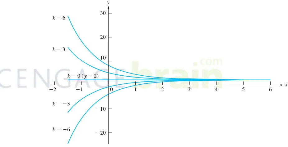
for all x. The integral curves ofy′+y=2 are graphs ofy=2+ke−x for different choices of
k. Some of these are shown in Figure 1.1.
x y
⫺20 ⫺10 10 20 30
0
⫺2 ⫺1 1 2 3 4 5 6
k⫽ 0 (y⫽ 2)
k⫽ 6
k⫽ 3
k⫽⫺3
k⫽⫺6
FIGURE 1.1 Integral curves ofy′+y=2fork=03−36, and−6.
EXAMPLE 1.2
It is routine to verify that the general solution of
y′+y x=e
x
is
y=1 xxe
x
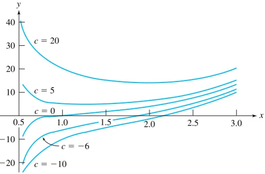
forx=0. Graphs of some of these integral curves, obtained by making choices forc, are shown in Figure 1.2.
c⫽ 0
c⫽ 20
c⫽ 5
c⫽⫺6
c⫽⫺10
y
40
30
20
10
0.5 1.0 1.5 2.0 2.5 3.0
⫺10
⫺20
x
FIGURE 1.2 Integral curves ofy′+1 xy=e
xforc=0520−6, and
−10.
We will see shortly how these general solutions are obtained. For the moment, we simply want to illustrate integral curves.
Although in simple cases integral curves can be sketched by hand, generally we need computer assistance. Computer packages such as MAPLE, MATHEMATICA and MATLAB are widely available. Here is an example in which the need for computing assistance is clear.
EXAMPLE 1.3
The differential equation
y′+xy=2
has general solution
yx=e−x2/2 x 0
2e2/2
d+ke−x2/2
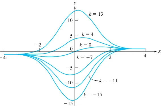
Figure 1.3 shows computer-generated integral curves corresponding tok=0, 4, 13, −7, −15 and−11.
1.1.4
The Initial Value Problem
The general solution of a first-order differential equation Fx y y′=0 contains an arbitrary constant, hence there is an infinite family of integral curves, one for each choice of the constant. If we specify that a solution is to pass through a particular pointx0 y0, then we must find that
particular integral curve (or curves) passing through this point. This is called an initial value problem. Thus, a first order initial value problem has the form
Fx y y′=0 yx
0=y0
k⫽ 0
k⫽ 13
k⫽ 4
k⫽⫺7
k⫽⫺15
k⫽⫺11
10
5
0
4 2
⫺5
⫺10
⫺15 ⫺4
⫺2
x y
FIGURE 1.3 Integral curves ofy′+xy=2fork=0413−7−15, and
−11.
EXAMPLE 1.4
Consider the initial value problem
y′+y=2 y1= −5
From Example 1.1, the general solution ofy′+y=2 is
y=2+ke−x
Graphs of this equation are the integral curves. We want the one passing through1−5. Solve forkso that
y1=2+ke−1= −5
obtaining
k= −7e
The solution of this initial value problem is
y=2−7ee−x
=2−7e−x−1 As a check,y1=2−7= −5
The effect of the initial condition in this example was to pick out one special integral curve as the solution sought. This suggests that an initial value problem may be expected to have a unique solution. We will see later that this is the case, under mild conditions on the coefficients in the differential equation.
1.1.5
Direction Fields
y
x
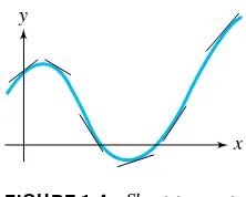
FIGURE 1.4 Short tangent segments suggest the shape of the curve.
The general first-order differential equation has the form
Fx y y′=0
Suppose we can solve fory′and write the differential equation as
y′=fx y
Here f is a known function. Suppose fx y is defined for all points x y in some region R of the plane. The slope of the integral curve through a given pointx0 y0 of Ris y′x0,
which equals fx0 y0. If we compute fx yat selected points inR, and draw a small line
segment having slopefx yat eachx y, we obtain a collection of segments which trace out the shapes of the integral curves. This enables us to obtain important insight into the behavior of the solutions (such as where solutions are increasing or decreasing, limits they might have at various points, or behavior asxincreases).
A drawing of the plane, with short line segments of slopefx ydrawn at selected points x y, is called adirection fieldof the differential equationy′=fx y. The name derives from the fact that at each point the line segment gives the direction of the integral curve through that point. The line segments are calledlineal elements.
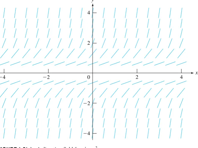
EXAMPLE 1.5
Consider the equation
y′=y2
Herefx y=y2, so the slope of the integral curve throughx yisy2. Select some points and,
through each, draw a short line segment having slopey2. A computer generated direction field
is shown in Figure 1.5(a). The lineal elements form a profile of some integral curves and give us some insight into the behavior of solutions, at least in this part of the plane. Figure 1.5(b) reproduces this direction field, with graphs of the integral curves through 01,02,03, 0−1,0−2and0−3.
By a method we will develop, the general solution ofy′=y2is
y= − 1 x+k
y
x
4
2
⫺2
⫺4
⫺2 0 2 4
⫺4
FIGURE 1.5(a) A direction field fory′=y2.
y
x
4
2
⫺2
⫺4
⫺2 0
2 4
⫺4
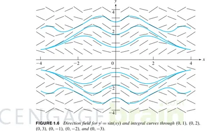
EXAMPLE 1.6
Figure 1.6 shows a direction field for
y′=sinxy
together with the integral curves through01,02,03,0−1,0−2and0−3. In this case, we cannot write a simple expression for the general solution, and the direction field provides information about the behavior of solutions that is not otherwise readily apparent.
y
x
⫺4 ⫺2
⫺2
⫺4 0 2 4
2 4
FIGURE 1.6 Direction field fory′=sinxyand integral curves through01,02, 03,0−1,0−2, and0−3.
With this as background, we will begin a program of identifying special classes of first-order differential equations for which there are techniques for writing the general solution. This will occupy the next five sections.
S E C T I O N 1 . 1
PROBLEMS
In each of Problems 1 through 6, determine whether the given function is a solution of the differential equation.
1. 2yy′=1 x=√x−1 forx >1
2. y′+y=0 x=Ce−x
3. y′= −2y+ex
2x forx >0 x= C−ex
2x
4. y′= 2xy
2−x2 forx= ±
√
2 x= C
x2−2
5. xy′=x−y x=x 2
−3
2x forx=0 6. y′+y=1 x=1+Ce−x
In each of Problems 7 through 11, verify by implicit differentiation that the given equation implicitly defines a solution of the differential equation.
7. y2
+xy−2x2
8. xy3
In each of Problems 12 through 16, solve the initial value problem and graph the solution.Hint:Each of these dif-ferential equations can be solved by direct integration. Use the initial condition to solve for the constant of integration.
12. y′=2x y2=1
13. y′=e−x y0=2
14. y′=2x+2 y−1=1
15. y′=4 cosxsinx y /2=0
16. y′=8x+cos2x y0= −3
In each of Problems 17 through 20 draw some lineal elements of the differential equation for −4≤x≤4,
−4≤y≤4. Use the resulting direction field to sketch a graph of the solution of the initial value problem. (These problems can be done by hand.)
17. y′=x+y y2=2
18. y′=x−xy y0= −1
19. y′=xy y0=2
20. y′=x−y+1 y0=1
In each of Problems 21 through 26, generate a direction field and some integral curves for the differential equation. Also draw the integral curve representing the solution of the initial value problem. These problems should be done by a software package.
21. y′=siny y1= /2
27. Show that, for the differential equationy′+pxy= qx, the lineal elements on any vertical linex=x0, with px0=0, all pass through the single point , where
DEFINITION 1.1 Separable Differential Equation
A differential equation is called separable if it can be written
y′=AxBy
In this event, we can separate the variables and write, in differential form,
1
By dy=Ax dx
whereverBy=0. We attempt to integrate this equation, writing
1
By dy=
Ax dx
EXAMPLE 1.7
y′=y2e−x is separable. Write
dy dx =y
2e−x
as
1
y2 dx=e
−xdx
fory=0. Integrate this equation to obtain
−1
y = −e −x
+k
an equation that implicitly defines the general solution. In this example we can explicitly solve fory, obtaining the general solution
y= 1
e−x−k
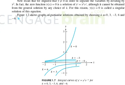
Now recall that we required that y=0 in order to separate the variables by dividing by y2. In fact, the zero functionyx=0 is a solution ofy′=y2ex, although it cannot be obtained from the general solution by any choice of k. For this reason,yx=0 is called a singular solution of this equation.
Figure 1.7 shows graphs of particular solutions obtained by choosingkas 0, 3,−3, 6 and
−6.
y
x k⫽ 0
k⫽⫺3
k⫽⫺6
k⫽ 3
k⫽ 6
⫺2 ⫺1 2
⫺1 3
2
1
1
FIGURE 1.7 Integral curves ofy′=y2e−xfor k=03−36, and−6.
EXAMPLE 1.8
x2y′=1+yis separable, and we can write
1 1+y dy=
1 x2 dx
The algebra of separation has required that x=0 andy= −1, even though we can putx=0 andy= −1 into the differential equation to obtain the correct equation 0=0.
Now integrate the separated equation to obtain
ln1+y = −1 x+k
This implicitly defines the general solution. In this case, we can solve foryxexplicitly. Begin by taking the exponential of both sides to obtain
1+y =eke−1/x=Ae−1/x
in which we have writtenA=ek. Sincekcould be any number,Acan be any positive number. Then
1+y= ±Ae−1/x=Be−1/x
in whichB= ±Acan be any nonzero number. The general solution is
y= −1+Be−1/x
in whichBis any nonzero number.
Now revisit the assumption that x=0 and y= −1. In the general solution, we actually obtain y= −1 if we allow B=0. Further, the constant function yx= −1 does satisfy x2y′=1+y. Thus, by allowingBto be any number, including 0, the general solution
yx= −1+Be−1/x
contains all the solutions we have found. In this example, y= −1 is a solution, but not a singular solution, since it occurs as a special case of the general solution.
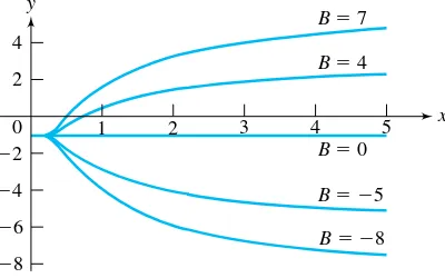
Figure 1.8 shows graphs of solutions corresponding toB= −8−504 and 7.
y
x
B⫽ 7
B⫽ 4
B⫽ 0
B⫽⫺5
B⫽⫺8
⫺2
⫺4
⫺6
⫺8 4
2
0 1 2 3 4 5
FIGURE 1.8 Integral curves ofx2y′=1+yfor B=047−5, and−8.
EXAMPLE 1.9
Solve the initial value problem
y′=y2e−x y1
=4
We know from Example 1.7 that the general solution ofy′=y2e−xis
yx= 1
e−x−k
Now we need to choosekso that
y1= 1
e−1−k=4
from which we get
k=e−1
−1
4
The solution of the initial value problem is
yx= 1
e−x+1 4−e−
1
EXAMPLE 1.10
The general solution of
y′=yx−1
2
y+3
is implicitly defined by
y+3 lny =1 3x−1
3
+k (1.3)
To obtain the solution satisfyingy3= −1, putx=3 andy= −1 into equation (1.3) to obtain
−1=1
32
3
+k
hence
k= −11 3
The solution of this initial value problem is implicitly defined by
y+3 lny =1 3x−1
3
−11
3
1.2.1
Some Applications of Separable Differential Equations
EXAMPLE 1.11
(The Mathematical Policewoman) A murder victim is discovered, and a lieutenant from the forensic science laboratory is summoned to estimate the time of death.
The body is located in a room that is kept at a constant 68 degrees Fahrenheit. For some time after the death, the body will radiate heat into the cooler room, causing the body’s temperature to decrease. Assuming (for want of better information) that the victim’s temperature was a “normal” 986 at the time of death, the lieutenant will try to estimate this time by observing the body’s current temperature and calculating how long it would have had to lose heat to reach this point.
According to Newton’s law of cooling, the body will radiate heat energy into the room at a rate proportional to the difference in temperature between the body and the room. IfTtis the body temperature at timet, then for some constant of proportionalityk,
T′t=k Tt−68
The lieutenant recognizes this as a separable differential equation and writes
1
T−68 dT=k dt
Upon integrating, she gets
lnT−68 =kt+C
Taking exponentials, she gets
T−68 =ekt+C=Aekt in whichA=eC. Then
T−68= ±Aekt=Bekt
Then
Tt=68+Bekt
Now the constantskandBmust be determined, and this requires information. The lieutenant arrived at 9:40 p.m. and immediately measured the body temperature, obtaining 944 degrees. Letting 9:40 be time zero for convenience, this means that
T0=944=68+B
and so B=264. Thus far,
Tt=68+264ekt
To determine k, the lieutenant makes another measurement. At 11:00 she finds that the body temperature is 892 degrees. Since 11:00 is 80 minutes past 9:40, this means that
T80=892=68+264e80k
Then
e80k
=212
264 so
80k=ln
212
264
and
k= 1 80ln
212
264
The lieutenant now has the temperature function:
Tt=68+264eln212/264t/80
In order to find when last time when the body was 986 (presumably the time of death), solve for the time in
Tt=986=68+264eln212/264t/80
To do this, the lieutenant writes
306 264 =e
ln212/264t/80
and takes the logarithm of both sides to obtain
ln
306
264
= t
80ln
212
264
Therefore the time of death, according to this mathematical model, was
t=80 ln306/264 ln212/264
which is approximately −538 minutes. Death occurred approximately 538 minutes before (because of the negative sign) the first measurement at 9:40, which was chosen as time zero. This puts the murder at about 8:46 p.m.
EXAMPLE 1.12
(Radioactive Decay and Carbon Dating) In radioactive decay, mass is converted to energy by radiation. It has been observed that the rate of change of the mass of a radioactive substance is proportional to the mass itself. This means that, ifmtis the mass at timet, then for some constant of proportionalitykthat depends on the substance,
dm dt =km
This is a separable differential equation. Write it as
1
mdm=k dt
and integrate to obtain
lnm =kt+c
Since mass is positive,m =mand
lnm=kt+c
Then
mt=ekt+c
Determination of A andk for a given element requires two measurements. Suppose at some time, designated as time zero, there areM grams present. This is called the initial mass. Then
m0=A=M
so
mt=Mekt
If at some later timeT we find that there areMT grams, then
mT=MT=Me kT
Then
ln
M
T
M
=kT
hence
k= 1 Tln
M
T
M
This gives uskand determines the mass at any time:
mt=MelnMT/Mt/T
We obtain a more convenient formula for the mass if we choose the time of the second measurement more carefully. Suppose we make the second measurement at that time T=H at which exactly half of the mass has radiated away. At this time, half of the mass remains, so MT=M/2 andMT/M=1/2. Now the expression for the mass becomes
mt=Meln1/2t/H
or
mt=Me−ln2t/H (1.4)
This number H is called the half-life of the element. Although we took it to be the time needed for half of the original amount M to decay, in fact, between any timest1 andt1+H,
exactly half of the mass of the element present att1will radiate away. To see this, write
mt1+H=Me−ln2t1+H/H
=Me−ln2t1/He−ln2H/H=e−ln2mt 1
=12mt1
Equation (1.4) is the basis for an important technique used to estimate the ages of certain ancient artifacts. The earth’s upper atmosphere is constantly bombarded by high-energy cosmic rays, producing large numbers of neutrons, which collide with nitrogen in the air, changing some of it into radioactive carbon-14, or14C. This element has a half-life of about 5,730 years.
Over the relatively recent period of the history of this planet in which life has evolved, the fraction of 14C in the atmosphere, compared to regular carbon, has been essentially constant.
This means that living matter (plant or animal) has injested14C at about the same rate over a
long historical period, and objects living, say, two million years ago would have had the same ratio of carbon-14 to carbon in their bodies as objects alive today. When an organism dies, it ceases its intake of14C, which then begins to decay. By measuring the ratio of14C to carbon
estimate of the time the organism was alive. This process of estimating the age of an artifact is calledcarbon dating. Of course, in reality the ratio of14C in the atmosphere has only been
approximately constant, and in addition a sample may have been contaminated by exposure to other living organisms, or even to the air, so carbon dating is a sensitive process that can lead to controversial results. Nevertheless, when applied rigorously and combined with other tests and information, it has proved a valuable tool in historical and archeological studies.
To apply equation (1.4) to carbon dating, useH=5730 and compute
ln2
H =
ln2
5730 ≈0000120968
in which ≈means “approximately equal” (not all decimal places are listed). Equation (1.4) becomes
mt=Me−0000120968t
Now suppose we have an artifact, say a piece of fossilized wood, and measurements show that the ratio of 14C to carbon in the sample is 37 percent of the current ratio. If we say that the
wood died at time 0, then we want to compute the time T it would take for one gram of the radioactive carbon to decay this amount. Thus, solve forT in
037=e−0000120968T
We find that
T= − ln037
0000120968≈8,219
years. This is a little less than one and one-half half-lives, a reasonable estimate if nearly 2 3 of
the14C has decayed.
EXAMPLE 1.13
(Torricelli’s Law) Suppose we want to estimate how long it will take for a container to empty by discharging fluid through a drain hole. This is a simple enough problem for, say, a soda can, but not quite so easy for a large oil storage tank or chemical facility.
We need two principles from physics. The first is that the rate of discharge of a fluid flowing through an opening at the bottom of a container is given by
dV
dt = −kAv
in whichVt is the volume of fluid in the container at time t,vtis the discharge velocity of fluid through the opening, Ais the cross sectional area of the opening (assumed constant), andkis a constant determined by the viscosity of the fluid, the shape of the opening, and the fact that the cross-sectional area of fluid pouring out of the opening is slightly less than that of the opening itself. In practice,kmust be determined for the particular fluid, container, and opening, and is a number between 0 and 1.
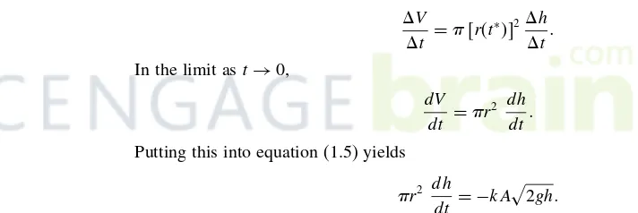
We also need Torricelli’s law, which states thatvtis equal to the velocity of a free-falling particle released from a height equal to the depth of the fluid at time t. (Free-falling means that the particle is influenced by gravity only). Now the work done by gravity in moving the particle from its initial point by a distance htis mght, and this must equal the change in the kinetic energy,1
2mv
2. Therefore,
18 18 ⫺h r
h
FIGURE 1.9
Putting these two equations together yields
dV
dt = −kA
2ght (1.5)
We will apply equation (1.5) to a specific case to illustrate its use. Suppose we have a hemispherical tank of water, as in Figure 1.9. The tank has radius 18 feet, and water drains through a circular hole of radius 3 inches at the bottom. How long will it take the tank to empty?
Equation (1.5) contains two unknown functions,Vtandht, so one must be eliminated. Let rt be the radius of the surface of the fluid at time t and consider an interval of time fromt0tot1=t0+t. The volumeV of water draining from the tank in this time equals the volume of a disk of thicknessh(the change in depth) and radiusrt∗, for some t∗between t0 andt1. Therefore
V = rt∗2
h
so
V
t = rt
∗2h
t
In the limit ast→0,
dV dt = r
2 dh
dt
Putting this into equation (1.5) yields
r2 dh
dt = −kA
2gh
NowV has been eliminated, but at the cost of introducingrt. However, from Figure 1.9,
r2
=182−18−h2
=36h−h2
so
36h−h2dh
dt = −kA
2gh
This is a separable differential equation, which we write as
36h−h2
h1/2 dh= −kA
2g dt
Takeg to be 32 feet per second per second. The radius of the circular opening is 3 inches, or
1
4 feet, so its area isA= /16 square feet. For water, and an opening of this shape and size,
the experiment givesk=08. The last equation becomes
36h1/2−h3/2
dh= −08
1
16
√
or
36h1/2−h3/2
dh= −04dt
A routine integration yields
24h3/2
Thusk=2268√2 andhtis implicitly determined by the equation
60h3/2
−h5/2
=2268√2−t
The tank is empty whenh=0, and this occurs whent=2268√2 seconds, or about 53 minutes, 28 seconds.
The last three examples contain an important message. Differential equations can be used to solve a variety of problems, but a problem usually does not present itself as a differential equation. Normally we have some event or process, and we must use whatever information we have about it to derive a differential equation and initial conditions. This process is called mathematical modeling. The model consists of the differential equation and other relevant information, such as initial conditions. We look for a function satisfying the differential equation and the other information, in the hope of being able to predict future behavior, or perhaps better understand the process being considered.
S E C T I O N 1 . 2
PROBLEMS
In each of Problems 1 through 10, determine if the dif-ferential equation is separable. If it is, find the general solution (perhaps implicitly defined). If it is not separa-ble, do not attempt a solution at this time.
1. 3y′=4x/y2
In each of Problems 11 through 15, solve the initial value problem.
16. An object having a temperature of 90 degrees Fahren-heit is placed into an environment kept at 60 degrees. Ten minutes later the object has cooled to 88 degrees. What will be the temperature of the object after it has been in this environment for 20 minutes? How long will it take for the object to cool to 65 degrees?
18. Assume that the population of bacteria in a petri dish changes at a rate proportional to the population at that time. This means that, ifPtis the population at timet, then
dP dt =kP
for some constantk. A particular culture has a popu-lation density of 100,000 bacteria per square inch. A culture that covered an area of 1 square inch at 10:00 a.m. on Tuesday was found to have grown to cover 3 square inches by noon the following Thursday. How many bacteria will be present at 3:00 p.m. the follow-ing Sunday? How many will be present on Monday at 4:00 p.m.? When will the world be overrun by these bacteria, assuming that they can live anywhere on the earth’s surface? (Here you need to look up the land area of the earth.)
19. Assume that a sphere of ice melts at a rate pro-portional to its surface area, retaining a spherical shape. Interpret melting as a reduction of volume with respect to time. Determine an expression for the vol-ume of the ice at any timet.
20. A radioactive element has a half-life of ln2weeks. Ife3 tons are present at a given time, how much will be left 3 weeks later?
21. The half-life of uranium-238 is approximately 45·109 years. How much of a 10-kilogram block of U-238 will be present 1 billion years from now?
22. Given that 12 grams of a radioactive element decays to 91 grams in 4 minutes, what is the half-life of this element?
CalculateI′x by differentiating under the integral sign, then letu=x/t. Show thatI′x= −2Ixand solve forIx. Evaluate the constant by using the stan-dard result that
0 e−t
2
dt=√ /2. Finally, evaluate I3.
24. Derive the fact used in Example 1.13 that vt=
2ght. Hint: Consider a free-falling particle hav-ing heighthtat timet. The work done by gravity in moving the particle from its starting point to a given point ismght, and this must equal the change in the kinetic energy, which is1/2mv2.
25. Calculate the time required to empty the hemispher-ical tank of Example 1.13 if the tank is positioned with its flat side down.
26. (Draining a Hot Tub) Consider a cylindrical hot tub with a 5-foot radius and height of 4 feet, placed on one of its circular ends. Water is draining from the tub through a circular hole 58 inches in diameter located in the base of the tub.
(a) Assume a valuek=06 to determine the rate at which the depth of the water is changing. Here it is useful to write
(b) Calculate the timeTrequired to drain the hot tub if it is initially full.Hint:One way to do this is to write
T=
0
H dt dh dh
(c) Determine how much longer it takes to drain the lower half than the upper half of the tub.Hint:Use the integral suggested in (b), with different limits for the two halves.
27. (Draining a Cone) A tank shaped like a right circular cone, with its vertex down, is 9 feet high and has a diameter of 8 feet. It is initially full of water.
(a) Determine the time required to drain the tank through a circular hole of diameter 2 inches at the vertex. Takek=06.
(b) Determine the time it takes to drain the tank if it is inverted and the drain hole is of the same size and shape as in (a), but now located in the new base.
28. (Drain Hole at Unknown Depth) Determine the rate of change of the depth of water in the tank of Problem 27 (vertex at the bottom) if the drain hole is located in the side of the cone 2 feet above the bottom of the tank. What is the rate of change in the depth of the water when the drain hole is located in the bottom of the tank? Is it possible to determine the location of the drain hole if we are told the rate of change of the depth and the depth of the water in the tank? Can this be done without knowing the size of the drain opening?
29. Suppose the conical tank of Problem 27, vertex at the bottom, is initially empty and water is added at the constant rate of /10 cubic feet per second. Does the tank ever overflow?
1.3
Linear Differential Equations
DEFINITION 1.2 Linear Differential Equation
A first-order differential equation is linear if it has the form
y′x+pxy=qx
Assume thatpandqare continuous on an intervalI(possibly the whole real line). Because of the special form of the linear equation, we can obtain the general solution onI by a clever observation. Multiply the differential equation byepx dxto get
epx dxy′x+pxepx dxy=qxepx dx
The left side of this equation is the derivative of the productyxepx dx, enabling us to write
d
dx yxe
px dx
=qxepx dx Now integrate to obtain
yxepx dx
= qxepx dxdx
+C
Finally, solve foryx:
yx=e−px dx qxepx dxdx+Ce−px dx (1.6) The functione
px dxis called anintegrating factorfor the differential equation, because
multi-plication of the differential equation by this factor results in an equation that can be integrated to obtain the general solution. We do not recommend memorizing equation (1.6). Instead, recognize the form of the linear equation and understand the technique of solving it by multiplying byepx dx.
EXAMPLE 1.14
The equation y′+y=sinx is linear. Herepx=1 andqx=sinx, both continuous for allx. An integrating factor is
edx orex. Multiply the differential equation byex to get
y′ex
+yex
=ex sinx
or
yex′=exsinx
Integrate to get
yex
=exsinx dx
=1
2e xsinx
−cosx+C
The general solution is
yx=1
EXAMPLE 1.15
Solve the initial value problem
y′=3x2
−y
x y1=5
First recognize that the differential equation can be written in linear form:
y′+1 xy=3x
2
An integrating factor ise1/x dx
=elnx
=x, forx >0. Multiply the differential equation byx to get
xy′+y=3x3
or
xy′=3x3
Integrate to get
xy=3 4x
4
+C
Then
yx=3 4x
3
+C
x
forx >0. For the initial condition, we need
y1=5=3
4+C
soC=17/4 and the solution of the initial value problem is
yx=3 4x
3
+174x
forx >0.
Depending onpandq, it may not be possible to evaluate all of the integrals in the general solution 1.6 in closed form (as a finite algebraic combination of elementary functions). This occurs with
y′+xy=2
whose general solution is
yx=2e−x2/2
ex2/2
dx+Ce−x2/2
We cannot write
ex2/2
y
x
⫺2 0 2 4
2 4
⫺4 ⫺2
⫺4
FIGURE 1.10 Integral curves ofy′+xy=2passing through02, 04,0−2, and0−5.
Linear differential equations arise in many contexts. Example 1.11, involving estimation of time of death, involved a separable differential equation which is also linear and could have been solved using an integrating factor.
EXAMPLE 1.16
(A Mixing Problem) Sometimes we want to know how much of a given substance is present in a container in which various substances are being added, mixed, and removed. Such problems are calledmixing problems, and they are frequently encountered in the chemical industry and in manufacturing processes.
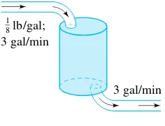
As an example, suppose a tank contains 200 gallons of brine (salt mixed with water), in which 100 pounds of salt are dissolved. A mixture consisting of 1
8 pound of salt per gallon is
flowing into the tank at a rate of 3 gallons per minute, and the mixture is continuously stirred. Meanwhile, brine is allowed to empty out of the tank at the same rate of 3 gallons per minute (Figure 1.11). How much salt is in the tank at any time?
3 gal/min lb/gal;
3 gal/min
1 8
FIGURE 1.11
Now letQtbe the amount of salt in the tank at time t. The rate of change ofQtwith time must equal the rate at which salt is pumped in, minus the rate at which it is pumped out. Thus
dQ
dt =(rate in)−(rate out)
=
1
8 pounds
gallon 3 gallons minute
−
Qt
200 pounds
gallon 3 gallons minute
=3
8− 3 200Qt
This is the linear equation
Q′t+ 3 200Q=
3 8
An integrating factor is e3/200 dt
=e3t/200. Multiply the differential equation by this factor to
obtain
Q′e3t/200+ 3 200e
3t/200
Q=3 8e
3t/200
or
Qe3t/200′
=38e3t/200
Then
Qe3t/200
=3
8 200
3 e
3t/200
+C
so
Qt=25+Ce−3t/200
Now
Q0=100=25+C
soC=75 and
Qt=25+75e−3t/200
As we expected, astincreases, the amount of salt approaches the limiting value of 25 pounds. From the derivation of the differential equation forQt, it is apparent that this limiting value depends on the rate at which salt is poured into the tank, but not on the initial amount of salt in the tank. The term 25 in the solution is called the steady-state part of the solution because it is independent of time, and the term 75e−3t/200 is the transient part. Ast increases,
S E C T I O N 1 . 3
PROBLEMS
In each of Problems 1 through 8, find the general solution. Not all integrals can be done in closed form.
1. y′−3
In each of Problems 9 through 14, solve the initial value problem.
15. Find all functions with the property that they-intercept of the tangent to the graph atx yis 2x2.
16. A 500-gallon tank initially contains 50 gallons of brine solution in which 28 pounds of salt have been dissolved. Beginning at time zero, brine containing 2 pounds of salt per gallon is added at the rate of 3 gallons per minute, and the mixture is poured out of the tank at the rate of 2 gallons per minute. How much salt is in the tank when it contains 100 gallons of brine? Hint:The amount of brine in the tank at timetis 50+t. 17. Two tanks are cascaded as in Figure 1.12. Tank 1 initially contains 20 pounds of salt dissolved in 100 gallons of brine, while tank 2 contains 150 gallons of brine in which 90 pounds of salt are dissolved. At time zero a brine solution containing 1
2 pound of salt per gallon is added to tank 1 at the rate of 5 gallons per minute. Tank 1 has an output that discharges brine into tank 2 at the rate of 5 gallons per minute, and tank 2 also has an output of 5 gallons per minute. De-termine the amount of salt in each tank at any timet. Also determine when the concentration of salt in tank 2 is a minimum and how much salt is in the tank at that time.Hint:Solve for the amount of salt in tank 1 at timetfirst and then use this solution to determine the amount in tank 2.
Tank 2 Tank 1
5 gal/min 5 gal/min
5 gal/min lb/gal
1 2
FIGURE 1.12 Mixing between tanks in Problem 17.
1.4
Exact Differential Equations
We continue the theme of identifying certain kinds of first-order differential equations for which there is a method leading to a solution.
We can write any first order equationy′=fx yin the form
Mx y+Nx yy′=0
For example, putMx y= −fx yandNx y=1. An interesting thing happens if there is a functionsuch that
x =Mx y and
In this event, the differential equation becomes
x +
y
dy dx=0
which, by the chain rule, is the same as
d
dx x yx=0
But this means that
x yx=C
withCconstant. If we now read this argument from the last line back to the first, the conclusion is that the equation
x y=C
implicitly defines a functionyxthat is the general solution of the differential equation. Thus, finding a function that satisfies equation (1.7) is equivalent to solving the differential equation.
Before taking this further, consider an example.
EXAMPLE 1.17
The differential equation
y′= − 2xy
3
+2
3x2y2+8e4y
is neither separable nor linear. Write it in the form
M+Ny′=2xy3
+2+
3x2y2
+8e4y
y′=0 (1.8)
with
Mx y=2xy3+2 and Nx y=3x2y2+8e4y
Equation (1.8) can in turn be written
M dx+N dy=2xy3
+2 dx+3x2y2
+8e4y dy
=0 (1.9)
Now let
x y=x2y3
+2x+2e4y
Soon we will see where this came from, but for now, observe that
x =2xy
3
+2=M and
y =3x
2
y2+8e4y=N
With this choice ofx y, equation (1.9) becomes
x dx+
y dy=0
or
The general solution of this equation is
x y=C
or, in this example,
x2y3
+2x+2e4y
=C
This implicitly defines the general solution of the differential equation (1.8). To verify this, differentiate the last equation implicitly with respect tox:
2xy3
+3x2y2y′+2+8e4y
y′=0
or
2xy3+2+3x2y2+8e4yy′=0
This is equivalent to the original differential equation
y′= − 2xy
3
+2
3x2y2+8e4y
With this as background, we will make the following definitions.
DEFINITION 1.3 Potential Function
A function is a potential function for the differential equationMx y+Nx yy′=0 on a regionRof the plane if, for eachx yinR,
x =Mx y and
y =Nx y
DEFINITION 1.4 Exact Differential Equation
When a potential function exists on a regionRfor the differential equationM+Ny′=0, then this equation is said to be exact onR.
The differential equation of Example 1.17 is exact (over the entire plane), because we exhibited a potential function for it, defined for allx y. Once a potential function is found, we can write an equation implicitly defining the general solution. Sometimes we can explicitly solve for the general solution, and sometimes we cannot.
Now go back to Example 1.17. We want to explore how the potential function that materialized there was found. Recall we required that
x =2xy
3
+2=M and
y =3x
2
Pick either of these equations to begin and integrate it. Say we begin with the first. Then integrate with respect tox:
x y=
x dx=
2xy3
+2
dx
=x2y3
+2x+gy
In this integration with respect toxwe heldyfixed, hence we must allow thatyappears in the “constant” of integration. If we calculate/x, we get 2xy2+2 for any functiongy.
Now we knowto within this functiong. Use the fact that we know/yto write
y =3x
2y2
+8e4y
=
yx
2y3
+2x+gy=3x2y2
+g′y
This equation holds ifg′y=8e4y, hence we may choosegy
=2e4y. This gives the potential function
x y=x2y3
+2x+2e4y
If we had chosen to integrate/yfirst, we would have gotten
x y=
3x2y2
+8e4y
dy
=x2y3
+2e4y
+hx
Herehcan be any function of one variable, because no matter howhxis chosen,
y
x2y3
+2e4y
+hx
=3x2y2
+8e4y
as required. Now we have two expressions for/x:
x =2xy
3
+2
=x
x2y3
+2e4y
+hx
=2xy3
+h′x
This equation forces us to choose h so that h′x=2, and we may therefore set hx=2x. This gives
x y=x2y3
+2e4y
+2x
as we got before.
Not every first-order differential equation is exact. For example, consider
If there were a potential function, then we would have
x =y
y =1
Integrate/x=ywith respect toxto getx y=xy+gy. Substitute this into/y=1 to get
yxy+gy=x+g
′y=1
But this can hold only ifg′y=1−x, an impossibility ifgis to be independent ofx. Therefore, y+y′=0 has no potential function. This differential equation is not exact (even though it is easily solved either as a separable or as a linear equation).
This example suggests the need for a convenient test for exactness. This is provided by the following theorem, in which a “rectangle in the plane” refers to the set of points on or inside any rectangle having sides parallel to the axes.
THEOREM 1.1 Test for Exactness
SupposeMx y,Nx y,M/y, andN/xare continuous for allx ywithin a rectangleR in the plane. Then,
Mx y+Nx yy′=0
is exact onRif and only if, for eachx yinR,
M
y =
N
x
Proof IfM+Ny′=0 is exact, then there is a potential functionand
x =Mx y and
y =Nx y
Then, forx yinR,
M
y =
y
x
=
2
yx=
2
xy =
x
y
=Nx
Conversely, supposeM/yandN/xare continuous onR. Choose anyx0 y0inRand define, forx yinR,
x y=
x
x0
M y0 d+
y
y0
Nx d (1.10)
Immediately we have, from the fundamental theorem of calculus,
since the first integral in equation (1.10) is independent ofy. Next, compute
x =
x
x
x0
M y0 d+
x
y
y0
Nx d
=Mx y0+
y
y0
N
xx d
=Mx y0+
y
y0
M
yx d
=Mx y0+Mx y−Mx y0=Mx y
and the proof is complete.
For example, consider againy+y′=0. HereMx y=yandNx y=1, so
N
x =0 and
M
y =1
throughout the entire plane. Thus,y+y′=0 cannot be exact on any rectangle in the plane. We saw this previously by showing that this differential equation can have no potential function.
EXAMPLE 1.18
Consider
x2
+3xy+4xy+2xy′=0
HereMx y=x2
+3xyandNx y=4xy+2x. Now N
x =4y+2 and M
y =3x
and
3x=4y+2
is satisfied by allx yon a straight line. However,N/x=M/ycannot hold for allx yin an entire rectangle in the plane. Hence this differential equation is not exact on any rectangle.
EXAMPLE 1.19
Consider
exsiny−2x+excosy+1 y′=0
WithMx y=exsiny−2xandNx y=excosy+1, we have
N x =e
xcosy
=M
y
for allx y. Therefore this differential equation is exact. To find a potential function, set
x =e
x
siny−2x and y =e
x
Choose one of these equations and integrate it. Integrate the second equation with respect toy:
x y=ex
cosy+1 dy
=ex
siny+y+hx
Then we must have
The general solution of the differential equation is defined implicitly by
ex
siny+y−x2
=C
Note of Caution:Ifis a potential function forM+Ny′=0,itself is not the solution. The general solution is defined implicitly by the equationx y=C.
S E C T I O N 1 . 4
PROBLEMS
In each of Problems 1 through 8, determine where (if any-where) in the plane the differential equation is exact. If it is exact, find a potential function and the general solution, perhaps implicitly defined. If the equation is not exact, do not attempt a solution at this time.
1. 2y2
In each of Problems 9 through 14, determine if the differ-ential equation is exact in some rectangle containing in its interior the point where the initial condition is given. If so, solve the initial value problem. This solution may be implicitly defined. If the differential equation is not exact, do not attempt a solution.
9. 3y4−1+12xy3y′=0 y1=2
In Problems 15 and 16, choose a constant so that the differential equation is exact, then produce a potential function and obtain the general solution.
15. 2xy3−3y−3x+x2y2−2yy′=0
16. 3x2+xy−x2y−1y′=0
1.5
Integrating Factors
“Most” differential equations are not exact on any rectangle. But sometimes we can multiply the differential equation by a nonzero functionx yto obtain an exact equation. Here is an example that suggests why this might be useful.
EXAMPLE 1.20
The equation
y2−6xy+3xy−6x2y′=0 (1.11)
is not exact on any rectangle. Multiply it byx y=yto get
y3
−6xy2
+3xy2
−6x2yy′=0 (1.12)
Wherevery=0, equations (1.11) and (1.12) have the same solution. The reason for this is that equation (1.12) is just
y
y2
−6xy+3xy−6x2y′ =0
and ify=0, then necessarilyy2−6xy+3xy−6x2y′=0.
Now notice that equation (1.12) is exact (over the entire plane), having potential function
x y=xy3
−3x2y2
Thus the general solution of equation (1.12) is defined implicitly by
xy3
−3x2y2
=C
and, wherevery=0, this defines the general solution of equation (1.11) as well.
To review what has just occurred, we began with a nonexact differential equation. We multiplied it by a functionchosen so that the new equation was exact. We solved this exact equation, then found that this solution also worked for the original, nonexact equation. The functiontherefore enabled us to solve a nonexact equation by solving an exact one. This idea is worth pursuing, and we begin by giving a name to.
DEFINITION 1.5
Let Mx y and Nx y be defined on a region R of the plane. Then x y is an integrating factor forM+Ny′=0 ifx y=0 for allx yinR, andM+Ny′=0 is exact onR.
How do we find an integrating factor for M+Ny′=0? Forto be an integrating factor, M+Ny′=0 must be exact (in some region of the plane), hence
x N=
in this region. This is a starting point. Depending on M andN, we may be able to determine from this equation.
Sometimes equation (1.13) becomes simple enough to solve if we try as a function of justxor justy.
EXAMPLE 1.21
The differential equation x−xy−y′=0 is not exact. Here M =x−xy and N = −1 and equation (1.13) is
x −=
y x−xy
Write this as
−x =x−xy
y−x
Now observe that this equation is simplified if we try to findas just a function ofx, because in this event/y=0 and we are left with just
x =x
This is separable. Write
1
d=x dx
and integrate to obtain
ln = 1 2x
2
Here we let the constant of integration be zero because we need only one integrating factor. From the last equation, choose
x=ex2/2
a nonzero function. Multiply the original differential equation byex2/2
to obtain
x−xyex2/2−ex2/2y′=0
This equation is exact over the entire plane, and we find the potential function x y= 1−yex2/2
. The general solution of this exact equation is implicitly defined by
1−yex2/2
=C
In this case, we can explicitly solve foryto get
yx=1−Ce−x2/2
and this is also the general solution of the original equationx−xy−y′=0.
EXAMPLE 1.22
Consider 2y2
−9xy+3xy−6x2y′=0. This is not exact. With M =2y2
−9xy and N =
3xy−6x2, begin looking for an integrating factor by writing equation (1.13):
x
3xy−6x2
=
y 2y
2
−9xy
This is
3xy−6x2
x+3y−12x=2y
2
−9xy
y+4y−9x (1.14)
If we attempt =x, then/y=0 and we obtain
3xy−6x2
x +3y−12x=4y−9x
which cannot be solved foras just a function ofx. Similarly, if we try=y, so/x=0, we obtain an equation we cannot solve. We must try something else. Notice that equation (1.14) involves only integer powers ofxandy. This suggests that we tryx y=xayb. Substitute this into equation (1.14) and attempt to chooseaandb. The substitution gives us
3axayb+1−6axa+1yb+3xayb+1−12xa+1yb=2bxayb+1−9bxa+1yb+4xayb+1−9xa+1yb
Assume thatx=0 andy=0. Then we can divide byxayb to get
3ay−6ax+3y−12x=2by−9bx+4y−9x
Rearrange terms to write
1+2b−3ay=−3+9b−6ax
Sincexandyare independent, this equation can hold for allxandyonly if
1+2b−3a=0 and −3+9b−6a=0
Solve these equations to obtaina=b=1. An integrating factor isx y=xy. Multiply the differential equation byxyto get
2xy3
−9x2y2
+3x2y2
−6x3yy′=0
This is exact with potential functionx y=x2y3−3x3y2. Forx=0 andy=0, the solution
of the original differential equation is given implicitly by
x2y3
−3x3y2
=C
The manipulations used to find an integrating factor may fail to find some solutions, as we saw with singular solutions of separable equations. Here are two examples in which this occurs.
EXAMPLE 1.23
Consider
2xy y−1−y
We can solve this as a separable equation, but here we want to make a point about integrating factors. Equation (1.15) is not exact, butx y=y−1/yis an integrating factor fory=0, a condition not required by the differential equation itself. Multiplying the differential equation byx yyields the exact equation
2x−y−1
y y
′=0
with potential functionx y=x2
−y+lnyand general solution defined by
x2
−y+lny =C fory=0
This is also the general solution of equation (1.15), but the method used has required that y=0. However, we see immediately that y=0 is also a solution of equation (1.15). This singular solution is not contained in the expression for the general solution for any choice ofC.
EXAMPLE 1.24
The equation
y−3−xy′=0 (1.16)
is not exact, butx y=1/xy−3is an integrating factor forx=0 and y=3, conditions not required by the differential equation itself. Multiplying equation (1.16) by x y yields the exact equation
1 x−
1 y−3y
′=0
with general solution defined by
lnx +C=lny−3
This is also the general solution of equation (1.16) in any region of the plane not containing the linesx=0 ory=3.
This general solution can be solved foryexplicitly in terms ofx. First, any real number is the natural logarithm of some positive number, so write the arbitrary constant asC=lnk, in whichkcan be any positive number. The equation for the general solution becomes
lnx +lnk=lny−3
or
lnkx =lny−3
But theny−3= ±kx. Replacing±kwithK, which can now be any nonzero real number, we obtain
y=3+Kx
1.5.1
Separable Equations and Integrating Factors
We will point out a connection between separable equations and integrating factors. The separable equationy′=AxByis in general not exact. To see this, write it as
AxBy−y′=0
so in the present context we haveMx y=AxByandNx y= −1. Now
x −1=0 and
y AxBy=AxB
′y
and in general AxB′y=0.
However,y=1/Byis an integrating factor for the separable equation. If we multiply the differential equation by 1/By, we get
Ax− 1
Byy ′=0
an exact equation because
x
− 1
By
=
y Ax=0
The act of separating the variables is the same as multiplying by the integrating factor 1/By.
1.5.2
Linear Equations and Integrating Factors
Consider the linear equationy′+pxy=qx. We can write this as pxy−qx+y′=0, so in the present context,Mx y=pxy−qxandNx y=1. Now
x 1=0 and
y pxy−qx=px
so the linear equation is not exact unless pxis identically zero. However, x y=epx dx is an integrating factor. Upon multiplying the linear equation by, we get
pxy−qxepx dx
+epx dxy′=0 and this is exact because
x e
px dx
=pxepx dx= y
pxy−qxepx dx
S E C T I O N 1 . 5
PROBLEMS
1. Determine a test involving M and N to tell when M+Ny′=0 has an integrating factor that is a func-tion ofyonly.
2. Determine a test to determine whenM+Ny′=0 has an integrating factor of the formx y=xayb for some constantsaandb.
3. Considery−xy′=0.
(a) Show that this equation is not exact on any rect-angle.
(b) Find an integrating factorxthat is a function ofxalone.
(c) Find an integrating factorythat is a function ofyalone.
In each of Problems 4 through 12, (a) show that the differ-ential equation is not exact, (b) find an integrating factor, (c) find the general solution (perhaps implicitly defined), and (d) determine any singular solutions the differential equation might have.
4. xy′−3y=2x3
5. 1+3x−e−2yy′=0
6. 6x2y+12xy+y2+6x2+2yy′=0
7. 4xy+6y2+2x2+6xyy′=0
8. y2+y−xy′=0
9. 2xy2+2xy+x2y+x2y′=0
10. 2y2
−9xy+3xy−6x2y′=0 (Hint: try x y= xayb)
11. y′+y=y4(Hint:tryx y=eaxyb)
12. x2y′+xy= −y−3/2 (Hint:tryx y=xayb)
In each of Problems 13 through 20, find an integrating factor, use it to find the general solution of the differen-tial equation, and then obtain the solution of the inidifferen-tial value problem.
13. 1+xy′=0 ye4
=0
14. 3y+4xy′=0 y1=6
15. 2y3−2+3xy2y′=0 y3=1
16. y1+x+2xy′=0 y4=6
17. 2xy+3y′=0 y0=4 (Hint:try=yaebx2
)
18. 2y1+x2
+xy′=0 y2=3 (Hint:try=xaebx2
)
19. sinx−y+cosx−y−cosx−yy′=0 y0=7 /6
20. 3x2y
+y3
+2xy2y′=0 y2=1
21. Show that any nonzero constant multiple of an inte-grating factor forM+Ny′=0 is also an integrating factor.
22. Letx ybe an integrating factor forM+Ny′=0 and suppose that the general solution is defined by x y=C. Show thatx yGx yis also an integrating factor, for any differentiable function G of one variable.
1.6
Homogeneous, Bernoulli, and Riccati Equations
In this section we will consider three additional kinds of first-order differential equations for which techniques for finding solutions are available.
1.6.1
Homogeneous Differential Equations
DEFINITION 1.6 Homogeneous Equation
A first-order differential equation is homogeneous if it has the form
y′=f y x