A DIVERSIFIED DEEP BELIEF NETWORK FOR HYPERSPECTRAL
IMAGE CLASSIFICATION
P. Zhong a, *, Z. Q. Gong a, C. Schönlieb b a
ATR Lab., School of Electronic Science and Engineering, National University of Defense Technology, Changsha, 410073, China-{zhongping, gongzhiqiang13}@nudt.edu.cn
b
Dept. of Applied Mathematics and Theoretical Physics, University of Cambridge, Wilberforce Road, Cambridge, CB3 0WA, UK –[email protected]
Commission VII, WG VII/4
KEY WORDS:Diversity, Deep Belief Network (DBN), Hyperspectral Image, Classification
ABSTRACT:
In recent years, researches in remote sensing demonstrated that deep architectures with multiple layers can potentially extract abstract and invariant features for better hyperspectral image classification. Since the usual real-world hyperspectral image classification task cannot provide enough training samples for a supervised deep model, such as convolutional neural networks (CNNs), this work turns to investigate the deep belief networks (DBNs), which allow unsupervised training. The DBN trained over limited training samples usually has many “dead” (never responding) or “potential over-tolerant” (always responding) latent factors (neurons), which decrease the DBN’s description ability and thus finally decrease the hyperspectral image classification performance. This work proposes a new diversified DBN through introducing a diversity promoting prior over the latent factors during the DBN pre-training and fine-tuning procedures. The diversity promoting prior in the training procedures will encourage the latent factors to be uncorrelated, such that each latent factor focuses on modelling unique information, and all factors will be summed up to capture a large proportion of information and thus increase description ability and classification performance of the diversified DBNs. The proposed method was evaluated over the well-known real-world hyperspectral image dataset. The experiments demonstrate that the diversified DBNs can obtain much better results than original DBNs and comparable or even better performances compared with other recent hyperspectral image classification methods.
* Corresponding author
1. INTRODUCTION
Many popular methods have been developed for hyperspectral image classification in the past several decades. One of the approaches in this context is the use of only spectral features in popular classifiers, such as multinomial logistic regression (MLR) (Zhong et al, 2008; Zhong and Wang, 2014), support vector machines (SVMs) (Melgani and Bruzzone, 2004), AdaBoost (Kawaguchi and Nishii, 2007), Gaussian process approach (Sun et al, 2014), random forest (Ham et al, 2005), graph method (Camps-Valls et al, 2007; Gao et al, 2014), conditional random field (CRF) (Zhong and Wang, 2010; Zhong and Wang, 2011), and so on. Most of the popular classifiers can be deemed as ‘shallow’ methods with only one or two processing layers. However, researches in literature of both computer vision and remote sensing demonstrated that deep architectures with more layers can potentially extract abstract and invariant features for better image classification (LeCun et al, 2015). This motivates exploring the use of deep learning for hyperspectral image representation and classification (Romero et al, 2015; Hu et al, 2015; Chen et al, 2015; Tao et al, 2015; Chen et al, 2015).
There are, however, significant challenges in adapting deep learning for hyperspectral image classification. The standard approache to real-world hyperspectral image classification is to
select some samples from a given image for classifier training, and then use the learned classifier to classify the remaining test samples in the same image (Zhong and Wang, 2010). This means that we usually do not have enough training samples to train the deep models. This problem is more obvious in completely supervised training of large scale of deep models, such as convolutional neural networks (CNNs).
A few methods have been proposed to partially deal with the problem to make the deep learning fit for hyperspectral image classification. The methods can be divided into two categories. The first one deals with the problem through developing new fully unsupervised learning method (Romero et al, 2015). The second one is generally to design special network structures, which can be effectively trained over a limited number of training samples or even naturally support unsupervised training (Hu et al, 2015; Chen et al, 2015; Tao et al, 2015; Chen et al, 2015). The deep belief network (DBN) (Chen et al, 2015) is such a model, which can be pre-trained through a unsupervised way at first, and then the available labelled training samples are used to fine-tune the pre-trained model though optimize a cost function defined over the labels of the training samples and their predictions. This directly follows the modules of the real-world hyperspectral image classification tasks. Therefore, this work will investigate the DBN model for hyperspectral image classification.
DBN is composed of several layers of latent factors, which can be deemed as neurons of neural networks. But the limited training samples in the real-world hyperspectral image classification task usually lead to many “dead” (never responding) or “potential over-tolerant” (always responding) latent factors (neurons) in the trained DBN. Therefore most of the computations are performed for the redundant latent factors, which will further decrease the DBN’s description ability. In this work we aim to keep the number of latent factors small to reduce the demand for the mount of training samples, meanwhile try to make them as expressive as a large set of latent factors. It is achieved by a new DBN training method, which diversifies the DBN through introducing a diversity promoting prior over the latent factors during training procedure. The diversity promoting prior will encourage latent factors to be uncorrelated, such that each latent factor focuses on modelling unique information, and all factors will be summed up to capture a large proportion of the information. The topic of diversifying latent factors to improve the models’ performances became popular in recent years. There are a few of available works investigating the diversity in several typical models or classifiers, such as k-means (Zou et al, 2012), Latent Dirichlet allocation (Zou et al, 2012), Gaussian mixture model (Zhong et al, 2015), hidden markov model (Qiao et al, 2015), distance metric (Xie et al, 2015) and restricted Boltzmann machine (RBM) (Xie et al, 2015; Xiong et al, 2015). To the authors’ knowledge, there is no work about the topic on diversifying deep model to improve the hyperspectral image classification. Our method presents the first such a solution. It should be mentioned that since DBN is actually the stacking of multiple RBMs, the methods in work (Xie et al, 2015) and (Xiong et al, 2015) to diversify the RBMs can give us basic theories about the layer-wise diversity of DBN, but the diversity in deep structure and corresponding diversifying method still need to be investigated comprehensively.
The rest of the paper is arranged as follows. The diversifying method of DBN in unsupervised pre-training procedure is proposed in Section 2. Section 3 develops the diversifying method of DBN in fine-tuning procedure. Section 4 utilizes the real-world hyperspectral image to evaluate the proposed method. Finally our technique is concluded and discussed in Section 5.
2. DIVERSIFY DBN IN PRE-TRAINING PROCEDURE 2.1 DBN for Spectral Representation
A DBN model is constructed with a hierarchical series of RBMs. An RBM at l -layer in DBN is an energy-based generative model that consists of a layer with I binary visible units
1, 2,...,
h .The energy of the joint configuration of the visible and hidden units
l, lThe RBM defines a joint probability over the units as
exp
, ;
where Z is the partition function
exp
, ;
Then the conditional distributions
l 1| l
jp h v and
l 1| l|
p v h can be easily computed (Chen et al, 2015).
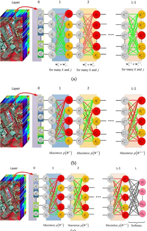
Fig.1(a) shows a typical DBN for deep feature learning from hyperspectral image. In DBN, the output of previous RBM is used as input data for a next RBM. Two adjacent layers have a full set of connections between them, but no two units in the same layer are connected. The input vector
0 0 0
1, 2,...,
T D
v v v could be the spectral signature of each pixel or the contextual features from neighbouring pixels. Every layer can output a feature of the input data, and the higher the layer is, the more abstract the feature is.
(a)
(b)
(c)
Fig. 1. Illustration of graph structure of DBN (a), diversified DBN in the unsupervised pre-training procedure (b) and supervised fine-tuning procedure (c). The binary latent variables are considered in this illustration. The nodes with yellow and red color mean that the latent variables have value 0 and 1 respectively.
2.2 Diversify DBN in Pre-training Procedure
The pre-training of DBN is implemented through a recursive greedy unsupervised learning procedure. The main idea is to train the RBMs, which are stacked to formulate the DBN, layer by layer using the Contrastive Divergence (CD) algorithm. However, the usual training method could lead to many “dead” (never responding) or “potential over-tolerant” (always responding) latent factors (neurons). See Fig. 1(a) for the illustration about this point. Therefore most of the computations are performed for the redundant latent factors, which decrease the DBN’s description ability.
We develop a new DBN training method to diversify the DBN model. The diversity means that the responses of latent units should be diverse. The proposed training method diversifies the latent units indirectly through diversifying the corresponding weight parameters layer by layer. The idea is to incorporate the diversity promoting conditions into the optimization of training objective. We propose to define a diversity promoting prior
lp w over the parameters and incorporate it into the learning procedure. one hidden unit. Their diversity can be informally described as how different each vector l
j
w is from others. There are many ways to measure the difference between vectors l
k difference measure is used to define diversity promoting prior (Xiong et al, 2015):
p w indicates that the weight vectors in l
w are more diverse.
To diversify the hidden units in RBM, we use the diversity prior described above to formulate the Maximum a posteriori (MAP) estimate of the weight vectors as
p X w is the likelihood of the given training data
1,2,..., promoting prior to diversify the latent units in the pre-training procedure. The optimization of (5) is equivalent to the maximization of log-posterior, and thus can be transformed to a constrained optimization:p X w is the log-likelihood of the given training data
The constrained optimization can be implemented as
T
2
2where is a parameter to control the weight of constraint in (6). Gradient ascent method can be used to implement the optimization (8) by computing the gradient
2
1IExact computation of the gradient l
jC X
w is intractable due
to the computation of an expectation w.r.t. the model's distribution (Hinton et al, 2006). In practice, gradient is often approximated using n-step CD, where the weights are updated as:
where recons represent the expectation w.r.t. the distribution after n steps of block Gibbs sampling starting at the data. More details can be found in (Hinton et al, 2006).
3. DIVERSIFY DBN IN FINE-TUNING PROCEDURE Fine-tuning DBN is equivalent to the training of a neural network with initialization of the parameters of the layers (besides the last softmax layer) as that of the (diversified) DBN. Fig. 1(c) shows the graph structure of the diversified DBN in the fine-tuning procedure.
The output of the j-thhidden unit of the l-th layer of the DBN DBN. For the last softmax layer, the output is
The International Archives of the Photogrammetry, Remote Sensing and Spatial Information Sciences, Volume XLI-B7, 2016where M is the number of classes and 1 , 2 ,..., L1
T
L L L L
m wm wm wJm
w
is the weight parameter vector for the m-th unit of the last layer. Equation (12) can be also deemed as the probability
| ,
Y y y y be the corresponding labels, where
1 2
ˆk xˆk,xˆk ,...,xˆkDT
x is a spectral signature with D bands, ˆk
y takes the label value from
1, 2,...,M
, K is the number of training samples. With the output of the DBN as the softmax, the MAP method fine-tunes the parameters of the DBN such that they minimize the negative log- posteriori
We consider only the diversity of weight parameters L1
W , and the parameters of different layers are usually assumed to be independent. Thus the normalized cost is written as
1
To diversify the latent units, the angle-based diversity prior (4) of the weight parameters are used. The objective function can be further written as
The constrained optimization can be implemented as minimizing the objective
and is a parameter to control the weight of constraint in (16). The stochastic gradient descent is used to optimize the objective function of (17), and gradient descent updates the parameters
1 2
implemented using the back propagation (BP) algorithm (Bishop, 1996). The gradient of the diversity promoting term
R W with respect to weight parameters can be computed as
14. EXPERIMENTAL RESULTS 4.1 Experimental Data set
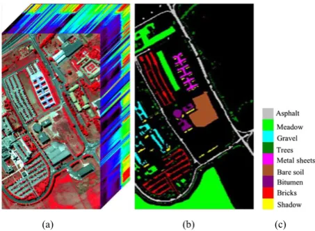
To validate effectiveness of the proposed diversifying method for hyperspectral image classification, we perform experiments over the real-world data cube named Pavia University. The data set was taken by a sensor known as the reflective optics system imaging spectrometer (ROSIS-3) over the city of Pavia, Italy. The image contains 610 × 340 pixels and 115 bands collected over 0.43-0.86 μm range of the electromagnetic spectrum. In the available data online, some bands were removed due to noise and the remaining 103 channels were used for the classification in this work. Nine land-cover classes were selected, which are shown in Fig. 2.
(a) (b) (c) Fig. 2. Pavia University data set. (a) Original image produced by the mixture of three bands. (b) Ground truth with nine classes. (c) Map color.
4.2 Experimental Setup
The available labelled samples are randomly divided into training set and test set to evaluate performance of the proposed method. For the Pavia University data set, all the nine land-cover classes were used to validate the proposed method, and for each class, 200 samples were randomly selected as the training samples. Table 1 shows the details of the training and test samples.
ID CLASS NAME TRAINING TEST
C1 Asphalt 200 6431
C2 Meadows 200 18449
C3 Gravel 200 1899
C4 Trees 200 2864
C5 Sheets 200 1145
C6 Bare soil 200 4829
C7 Bitumen 200 1130
C8 Bricks 200 3482
C9 Shadows 200 747
Total 1800 40976
Table 1 Number of training and test samples used in the Pavia University data set.
The model structure is one of the important factors to determine the performance of DBN. Generally, if given sufficient training samples, the DBN with more layers could have more abilities to represent the input data. For the limited training samples in our tasks and in consideration of the computational complexity, the structure of DBN is 103-50-…-50-9. Details about the effects of the structures of DBNs on the performances and the selection of structures can be found in (Chen et al, 2015). The parameter in the diversifying method is set to 103. To make the description clear, in the later contents the D-DBN-P is used to denote the DBN model diversified in only pre-training procedure, while the model diversified in pre-training procedure at first and then fine-tuning procedure is denoted as D-DBN-PF.
4.3 General Performances
1) Diversity of the Learned Models: Fig. 3 shows the examples
of diversified weight parameters over the Pavia University data set. For the page of limitation, only the results of the second layer are presented here. The learned parameters of the original DBN are also given for the comparisons. Inspecting the learned weight parameters of the original and diversified DBNs can demonstrate that at the same layer, the learned weight parameters through the proposed diversifying method show more diversity than that of the original DBN: there are more different rows in the diversified weight matrix.
(a) (b) (c)
Fig. 3. Example results of the learned weight parameters over the Pavia University data set: (a) is the learned weight parameters of the second layer of original DBN, (b) and (c) are the weights diversified by DBN-P and D-DBN-PF respectively.
2) The Classification Results: Table 2 shows the classification
results from the proposed diversified DBNs, where the structure is 103-50-50-50-50-9. The effects of the structures on the classification performance will be demonstrated later. In order to carry out quantitative evaluation, we computed average values from overall accuracies (OAs), average accuracies (AAs), and Kappa statistics (Kappa) of ten run of trainings and tests.
The D-DBN-PF obtained 93.11% OA and 93.92% AA, which are higher than 92.05% and 93.07 obtained by D-DBN-P. Table 2 also shows that the D-DBN-PF also obtained better Kappa measure than D-DBN-P. In addition, both the D-DBN-PF and D-DBN-P obtained better results than that of original DBN. To sum up, the diversifying learning in both the pre-training and fine-tuning procedures have obvious positive effects on the classification performances.
METHODS DBN D-DBN-P D-DBN-PF
CL
A
S
S
P
E
RCE
N
T
A
G
E
A
CCU
RA
CY
[
%
]
C1 87.37 88.03 89.58 C2 92.10 93.01 93.93 C3 85.57 87.36 88.41 C4 95.11 95.29 95.64 C5 99.74 99.56 99.56 C6 91.94 92.83 93.87 C7 92.21 92.74 93.19 C8 87.02 88.77 91.07
C9 100 100 100
OA[%] 91.18 92.05 93.11 AA[%] 92.34 93.07 93.92 KAPPA 0.8828 0.8942 0.9082 Table 2 Classification accuracies of DBN, D-DBN-P and D-DBN-PF over Pavia University data set.
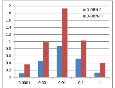
3) Classification Performances with Different Values of :
As mentioned in Section II, is regularization parameter, which controls the diversity of the learned priors: the larger is
, the greater is diversity. Moreover, the change of model diversity will further affect classification performance. Fig. 4 shows the behaviours of on OA improvements of D-DBN-P and D-DBN-PF over the original DBN. We can safely draw the conclusion from the figure that the larger is the value, the better is the classification performance, but excessively large values of will decrease classification performance. We can select favourable hyperparameter value to satisfy task’s specific requirements about the balance between model diversity and classification performance. In addition, in AA and Kappa measures the methods also show similar tendencies.
Fig. 4 Effects of parameter on the classification performances of proposed diversified DBNs. The figure shows improvements of results (OA(%)) of D-DBN-P and D-DBN-PF over original DBN.
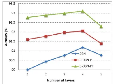
4) Classification Performances with Different Number of
Layers: The merits of deep learning methods derive mainly
from the increase of models’ depth, especially when sufficient training samples are provided. A set of experiments were designed to demonstrate this point. In addition, we will further investigate the performance of proposed diversifying method with the increase of models’ depth. Fig. 5 shows the classification results of DBN and the proposed D-DBN-P and D-DBN-PF. Experiments show that depth does help to improve classification accuracy. However, with only limited training samples available, too deep models will act inversely. The best depths are 4 for Pavia University data set. Moreover, the figure also shows that the proposed diversifying methods have higher performance improvements when the models have less layers.
Fig. 5. Classification accuracies versus numbers of layers for the Pavia University data set.
4.4 Comparisons with Other Recent Methods
To thoroughly evaluate the performance of the proposed methods, we ran several sets of experiments to compare them with the most recent results in hyperspectral image classification. Table 3 shows the details about the comparisons.
METHODS SVM-KAPPA 0.8771 0.9006 0.8828 0.8942 0.9082 Table 3 Classification accuracies of different methods.
1) Comparison to SVM. SVM-based method can be deemed as the benchmark ‘shallow’ hyperspectral image classification method. SVM-based method was trained and tested on same training and test data sets with the sizes presented in Table 1. The results in terms of classification accuracies provided by SVM-Poly and our methods are summarized in Table 3. The SVM-Poly obtained the classification result with OA, AA and
Kappa as 90.73%, 92.23% and 0.8771, while the proposed D-DBN-PF method obtained the better result with OA, AA and Kappa as 93.11%, 93.92% and 0.9082. Since the SVM-Poly is a typical ‘shallow’ classifier, thus the comparison between the results demonstrated that the DBN representations from the deep learning can benefit the hyperspectral image classification.
2) Comparison to CNN. CNNs are biologically inspired and
multilayer classes of deep learning models. They have demonstrated excellent performance on various visual tasks, including the classification of common two-dimensional images. Work (Hu et al, 2015) further introduced the CNN into the hyperspectral image classification and produced very promising results. Therefore, we further compare our method with the CNN. The architecture of the proposed CNN contains five layers, including the input layer, the convolutional layer, the max pooling layer, the full connection layer, and the output layer.
Table 3 shows the classification results of the CNNs and our proposed methods. For the fair comparison, our method was performed under the experimental setup same as that in work (Hu et al, 2015). Moreover, we used directly the results from work (Hu et al, 2015). However, only partial results corresponding to the evaluations in this work have been presented in work (Hu et al, 2015). Work (Hu et al, 2015) provided only the OA, and thus we calculated the AA and Kappa using the available results in work (Hu et al, 2015). The results show that the proposed models produced better results than that of CNNs. This means that besides the deep representation of the spectral observations, the model’s diversity also plays a very important role to improve the hyperspectral image classification.
5. CONCLUSION AND DISCUSSION
This work presented a diversifying method to improve the DBNs’ performance on description and classification of hyperspectral images. The new diversified DBNs were obtained through introducing a diversity promoting prior over the latent factors during two training procedures: the unsupervised pre-training and supervised fine-tuning. The introduced diversity prior encouraged the latent factors to be uncorrelated, such that each latent factor focuses on modelling unique information. Experiments were performed with real-world hyperspectral data cube. The results showed that the diversified DBNs obtained much better results than original DBNs did and comparable or even better performances compared with other recent hyperspectral image classification methods.
The experimental results of current form also indicate several future works. At first, the simple diversity promoting prior in (4) are used in this work. Other advanced diversity promoting prior could show more favourable properties in diversifying DBN. Secondly, the theory analysis of the performance improvement from model’s diversity is also an important future topic. Finally, it is worthy to investigate the proposed diversifying method for other models and applications.
ACKNOWLEDGEMENTS
This research was conducted with support of the Natural Science Foundation of China under Grant 61271439, A Foundation for the Author of National Excellent Doctoral Dissertation of P. R. China (FANEDD) under Grant 201243, Program for New Century Excellent Talents in University under The International Archives of the Photogrammetry, Remote Sensing and Spatial Information Sciences, Volume XLI-B7, 2016
Grant NECT-13-0164 and Chinese Scholarship Council under Grant 201407820015.
REFERENCES
Bishop C. M., 1996. Neural networks for pattern recognition. Oxford University Press.
Camps-Valls G., Marsheva T. V. B., and Zhou D., 2007. Semi-supervised graph-based hyperspectral image classification. IEEE Transactions on Geoscience and Remote Sensing, 45(10), pp. 3044-3054.
Chen Y., Lin Z., Zhao X., Wang G., and Gu Y., 2014. Deep learning-based classification of hyperspectral data. IEEE Journal of Selected Topics in Applied Earth Observations and Remote Sensing, 7(6), pp. 2094-2107.
Chen Y., Zhao X., and Jia X., 2015. Spectral-spatial classification of hyperspectral data based on deep belief network. IEEE Journal of Selected Topics in Applied Earth Observations and Remote Sensing, 8(6), pp. 2381-2392. Gao Y., Ji R., Cui P., Dai Q., and Hua G., 2014. Hyperspectral image classification through bilayer graph-based learning. IEEE Transactions on Image Processing, 23(7), pp. 2769-2778. Ham J., Chen Y., Crawford M. M., and Ghosh J., 2005. Investigation of the random forest framework for classification of hyperspectral data. IEEE Transactions on Geoscience and Remote Sensing, 43(3), pp. 492-501.
Hinton G. E., Osindero S., and Teh Y., 2006. A fast learning algorithm for deep belief nets. Neural Computation, 18, pp. 1527-1554.
Hu W., Huang Y., Wei L., Zhang F., and Li H., 2015. Deep convolutional neural networks for hyperspectral image classification. Journal of Sensors, Article ID: 258619, 12 pages. Kawaguchi S. and Nishii R., 2007. Hyperspectral image classification by bootstrap AdaBoost with random decision Stumps. IEEE Transactions on Geoscience and Remote Sensing, 45(11), pp. 3845-3851.
LeCun Y., Bengio Y., and Hinton G., 2015. Deep learning. Nature, 521, pp. 436-444.
Melgani F. and Bruzzone L., 2004. Classification of hyperspectral remote sensing images with support vector machines. IEEE Transactions on Geoscience and Remote Sensing, 42(8), pp. 1778-1790.
Qiao M., Bian W., Xu R. Y. D., and Tao D., 2015. Diversified hidden markov models for sequential labelling. IEEE Transactions on Knowledge and Data Engineering, 27(11), pp.2947-2960,
Romero A., Gatta C., and Camps-Valls G., 2016. Unsupervised deep feature extraction for remote sensing image classification. IEEE Transactions on Geoscience and Remote Sensing, 54(3):1349-1362.
Sun S., Zhong P., Xiao H., and Wang R., 2014. Active learning with Gaussian process classifier for hyperspectral image classification. IEEE Transactions on Geoscience and Remote Sensing, 53(4), pp. 1746-1760.
Tao C., Pan H., Li Y., and Zou Z., 2015. Unsupervised spectral-spatial feature learning with stacked sparse autoencoder for hyperspectral imagery classification. IEEE Geoscience and Remote Sensing Letter, 12(12), pp. 2438-2442.
Xiong H., Rodríguez-Sánchez A. J., Szedmak S., and Piater J., 2015. Diversity priors for learning early visual features. Frontiers in Computational Neuroscience, 9(Article 104), pp.1-11.
Xie P., Deng Y., Xing E. P., 2015. Diversifying restricted Boltzmann machine for document modelling. in Proc. ACM SIGKDD International Conference on Knowledge Discovery and Data Mining, pp.1315-1324.
Zhong P., Peng N., and Wang R., 2015. Learning to diversify patch-based priors for remote sensing image restoration, IEEE Journal of Selected Topics in Applied Earth Observations and Remote Sensing, 8(11), pp.5225-5245.
Zhong P. and Wang R., 2010. Learning conditional random fields for classification of hyperspectral images. IEEE Transactions on Image Processing, 19(7), pp. 1890-1907. Zhong P. and Wang R., 2011. Modeling and classifying hyperspectral imagery by CRFs with sparse higher order potentials. IEEE Transactions on Geoscience and Remote Sensing, 49(2), pp. 688-705.
Zhong P. and Wang R., 2014. Jointly learning the hybrid CRF and MLR model for simultaneous denoising and classification of hyperspectral imagery. IEEE Transactions on Neural Networks and Learning Systems, 25(7), pp. 1319-1334.
Zhong P., Zhang P., and Wang R., 2008. Dynamic learning of sparse multinomial logistic regression for feature selection and classification of hyperspectral data. IEEE Geoscience and Remote Sensing Letter, 5(2), pp. 280-284.
Zou J. Y. and Adams R. P., 2012. Priors for diversity in generative latent variable models. in Proc. Neural Information Processing Systems, pp. 2996-3004.