AUTOMATIC CAMERA ORIENTATION AND STRUCTURE RECOVERY WITH
SAMANTHA
R. Gherardi, R. Toldo, V. Garro, A. Fusiello
Dipartimento di Informatica, Universit`a di Verona Strada Le Grazie 15, 37134 Verona (Italy)
KEY WORDS:Structure and Motion, Autocalibration, Model acquisition.
ABSTRACT:
SAMANTHAis a software capable of computing camera orientation and structure recovery from a sparse block of casual images without human intervention. It can process both calibrated images or uncalibrated, in which case an autocalibration routine is run. Pictures are organized into a hierarchical tree which has single images as leaves and partial reconstructions as internal nodes. The method proceeds bottom up until it reaches the root node, corresponding to the final result. This framework is one order of magnitude faster than sequential approaches, inherently parallel, less sensitive to the error accumulation causing drift. We have verified the quality of our reconstructions both qualitatively producing compelling point clouds and quantitatively, comparing them with laser scans serving as ground truth.
1 INTRODUCTION
Three dimensional (3D) content is pervasive in most forms of dig-ital media, feeding the need for ubiquitous, effortless acquisition of 3D models. In this article we describeSAMANTHA, an auto-matic, robust software that can compute camera orientation and scene structure from a sparse block of casual (unconstrained) dig-ital images. Picture datasets are easy to capture, process and up-date. They have better resolution, contrast, definition of the video that can be produced with equally priced equipment. Pictures have also inferior requirements for storage and globally lower costs for production, maintenance and processing. Images are therefore the preferred way for ubiquitous, low cost acquisition of quality 3D data.
In Computer Vision the problem of recovering camera (exter-nal) orientation and scene 3D structure from images is known
asStructure and Motion. If the internal orientation is unknown
it must be computed as well and the problem becomes
uncali-brated.
Relevant literature comprises several Structure and Motion (SaM) pipelines that process images in batch and handle the reconstruc-tion process making no assumpreconstruc-tions on the imaged scene and on the acquisition rig (Brown and Lowe, 2005, Kamberov et al., 2006, Snavely et al., 2006, Vergauwen and Gool, 2006, Irschara et al., 2007).
The main issue to be solved in this context is the scalability of the SaM pipeline. This prompted a quest for efficiency that has explored several different solutions: the most successful have been those aimed at reducing the impact of the bundle adjustment phase, which – with feature extraction – dominates the computa-tional complexity.
A class of solutions that have been proposed are the so-called
partitioning methods(Fitzgibbon and Zisserman, 1998). They
reduce the reconstruction problem into smaller and better con-ditioned subproblems which can be effectively optimized. The subproblems can be selected analytically as in (Steedly et al., 2003), where spectral partitioning has been applied to SaM, or they can emerge from the underlying 3D structure of the prob-lem, as described in (Ni et al., 2007). The computational gain of
such methods is obtained by limiting the combinatorial explosion of the algorithm complexity as the number of images and feature points increases.
A second strategy is to select a subset of the input images and fea-ture points that subsumes the entire solution. Hierarchical sub-sampling was pioneered by (Fitzgibbon and Zisserman, 1998), using a balanced tree of trifocal tensors over a video sequence. The approach was subsequently refined by (Nist´er, 2000), adding heuristics for redundant frames suppression and tensor triplet se-lection. In (Shum et al., 1999) the sequence is divided into seg-ments, which are resolved locally. They are subsequently merged hierarchically, eventually using a representative subset of the seg-ment frames. A similar approach is followed in (Gibson et al., 2002), focusing on obtaining a well behaved segment subdivi-sion and on the robustness of the following merging step. The advantage of these methods over their sequential counterparts lays in the fact that they improve error distribution on the entire dataset and bridge over degenerate configurations. Anyhow, they work for video sequences, so they cannot be applied to unordered, sparse images.
A recent paper (Snavely et al., 2006) that works with sparse data-sets describes a way to select a subset of images whose recon-struction provably approximates the one obtained using the entire set. This considerably lowers the computational requirements by controllably removing redundancy from the dataset. Even in this case, however, the images selected are processed incrementally. Moreover, this method does not avoid computing the epipolar ge-ometry betweenallpairs of images.
A third solution is covered in literature, orthogonal to the afore-mentioned approaches. In (Agarwal et al., 2009), the computa-tional complexity of the reconstruction is tackled by throwing ad-ditional computational power to the problem. Within such frame-work, the former algorithmical challenges are substituted by load balancing and subdivision of reconstruction tasks. Such direc-tion of research strongly suggest that the current monolithical pipelines should be modified to accommodate ways to parallelize and optimally split the workflow of reconstruction tasks.
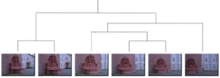
re-construction proceeding from leaves to the root. Partial recon-structions correspond to internal nodes, whereas images are stored in the leaves (see Fig. 1). This scheme provably cuts the compu-tational complexity by one order of magnitude (provided that the dendrogram is well balanced) and achieves scalability by parti-tioning the problem into smaller instances and combining them hierarchically in a inherently parallelizable way. It is also less sensible to typical problems of sequential approaches, namely sensitivity to initialization (Thorm¨ahlen et al., 2004) and drift (Cornelis et al., 2008). This approach has some analogy with (Schaffalitzky and Zisserman, 2002), where a spanning tree is built to establish in which order the images must be processed. After that, however, the images are processed in a standard incre-mental way.
Figure 1: An example of dendrogram for a 6 views set.
Most existing pipelines either assumes known internal parame-ters (Brown and Lowe, 2005, Irschara et al., 2007), or constant internal parameters (Vergauwen and Gool, 2006, Kamberov et al., 2006), or relies on EXIF data plus external informations (camera CCD dimensions) (Snavely et al., 2006). Another unique fea-ture ofSAMANTHAis the capability of dealing with uncalibrated images with varying internal parameters and no ancillary infor-mation, as it leverages on a a novel auto-calibration procedure robust enough to be applied in a real context.
The remainder of this article is organized as follows. The next section outlines the matching stage, then Sec. 3 describes the way the hierarchical cluster tree is built. Section 4 presents the hier-archical approach to structure and motion recovery, whereas the autocalibration strategy is explained in Sec. 5. We will then de-scribe the online image orientation stage in Sec. 6. Experimental detailed in Sec. 7, and finally conclusions are drawn in Sec. 8.
2 KEYPOINT MATCHING
In this section we describe the stage ofSAMANTHAthat is de-voted to the automatic extraction and matching of keypoints among all thenavailable images. Its output is to be fed into the geomet-ric stage, that will perform the actual reconstruction.
The objective is to identify in a computationally efficient way im-ages that potentially share a good number of keypoints, instead of trying to match keypoints between every image pair (they are O(n2
)). We follow the approach of (Brown and Lowe, 2003). SIFT (Lowe, 2004) keypoints are extracted in allnimages. In this culling phase we consider only a constant number of descrip-tors in each image (300 in our experiments, where a typical image contains thousands of SIFT keypoints). Then, each keypoint de-scription is matched to its�nearest neighbors in feature space (we use�= 8). This can be done inO(nlogn)time by using a k-d tree to find approximate nearest neighbors (we used the ANN library (Mount and Arya, 1996)). A 2D histogram is then built that registers in each bin the number of matches between the cor-responding views. Every image will be matched only to them images that have the greatest number of keypoints matches with
it (we usem = 8). Hence, the number of images to match is O(n), beingmconstant.
Matching follows a nearest neighbor approach (Lowe, 2004), with rejection of those keypoints for which the ratio of the nearest neighbor distance to the second nearest neighbor distance is greater than a threshold (set to1.5in our experiments).
Homographies and fundamental matrices between pairs of match-ing images are then computed usmatch-ing MSAC (Torr and Zisserman, 2000). Leteibe the residuals after MSAC, the final set of inliers
are those points such that
|ei−medjej|<3.5σ
∗
, (1)
whereσ∗
is a robust estimator of the scale of the noise:
σ∗= 1.4826 medi|ei−medjej|. (2)
This outlier rejection rule is called X84 in (Hampel et al., 1986).
The model parameters are eventually re-estimated on this set of inliers via least-squares minimization of the (first-order approxi-mation of the) geometric error (Luong and Faugeras, 1996, Chum et al., 2005).
The more likely model (homography or fundamental matrix) is selected according to the Geometric Robust Information Criterion (GRIC) (Torr, 1997). Finally, if the number of remaining matches between two images is less than a threshold (computed basing on a statistical test as in (Brown and Lowe, 2003)) then they are discarded.
Keypoints matching in multiple images are connected intotracks, rejecting as inconsistent those tracks in which more than one key-point converges (Snavely et al., 2006) and those shorter than three frames.
3 VIEWS CLUSTERING
The second stage ofSAMANTHAconsists in organizing the avail-able views into a hierarchical cluster structure that will guide the reconstruction process.
Algorithms for image views clustering have been proposed in lit-erature in the context of reconstruction (Schaffalitzky and Zis-serman, 2002), panoramas (Brown and Lowe, 2003), image min-ing (Quack et al., 2008) and scene summarization (Simon et al., 2007). The distance being used and the clustering algorithm are application-specific.
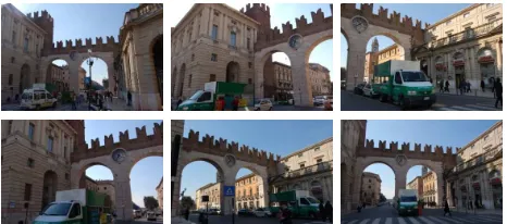
The method starts from an affinity matrix among views, com-puted using the following measure, that takes into account the number of common keypoints and how well they are spread over the images:
whereSiandSj are the set of matching keypoints in imageIi
andIjrespectively,CH(·)is the area of the convex hull of a set
of points andAi (Aj) is the total area of the image. Figure 2
shows an example of the neighborhood defined by this affinity.
Figure 2: An example of one image (top left) from “Piazza Bra” and its five closest neighbors according to the affinity defined in Eq. 3.
way the distance between clusters is computed produces differ-ent flavors of the algorithm, namely the simple linkage, complete linkage and average linkage (Duda and Hart, 1973). We selected
thesimple linkagerule: the distance between two clusters is
de-termined by the distance of the two closest objects (nearest neigh-bors) in the different clusters.
Simple linkage clustering is appropriate to our case because: i) the clustering problemper seis fairly simple, ii) nearest neigh-bors information is readily available with ANN and iii) it pro-duces “elongated” or “stringy” clusters which fits very well with the typical spatial arrangement of images sweeping a certain area or a building.
This procedure allows to decrease the computational complexity with respect to a sequential SaM pipeline, fromO(n5
)toO(n4
) in the best case (see (Gherardi et al., 2010) for a complete proof), i.e. when the tree is well balanced (nis the number of views). If the tree is unbalanced this computational gain vanishes. It is therefore crucial to enforce the balancing of the tree and this is the goal of the technique that we shall describe in this section.
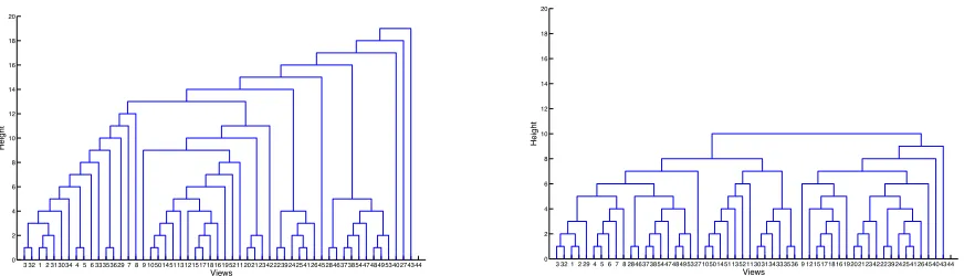
In order to produce better balanced trees and approximate best-case complexity, we modify the agglomerative clustering strategy as follows: starting from all singletons, each sweep of the algo-rithm merges the pair with the smallest cardinality among the� closest pair of clusters. The distance is computed according to the simple linkage rule. The cardinality of a pair is the sum of the cardinality of the two clusters.
In this way we are softening the “closest first” agglomerative cri-terion by introducing a competing “smallest first” principle that tends to produce better balanced dendrograms. The amount of balancing is regulated by the parameter�: when� = 1this is the standard agglomerative clustering with no balancing; when � ≥ n/2(nis the number of views) a perfect balanced tree is obtained, but the clustering is poor, since distance is largely dis-regarded. We found in our experiments (see Sec. 7) that a good compromise is�= 5. An example is shown in 3. The height of the tree is reduced from 14 to 9 and more initial pairs are present in the dendrogram on the right. Computational complexity de-crease accordingly.
Extra care must be taken when building clusters of cardinality two. These are pair of images from which the reconstruction will start, hence pairs related by homographies should be avoided. This is tantamount to say that the fundamental model must ex-plain the data far better than an homography, and this can be im-plemented by considering the GRIC, as in (Pollefeys et al., 2002). We therefore modify the linkage strategy so that two viewsiand viewjare allowed to merge in a cluster only if:
gric(Fi,j)< αgric(Hi,j) withα≥1, (4)
wheregric(Fi,j)andgric(Hi,j)are the GRIC scores obtained by
the fundamental matrix and the homography matrix respectively (we usedα = 1.2). If the test fail, consider the second closest elements and repeat.
4 HIERARCHICAL STRUCTURE AND MOTION
The dendrogram produced by the clustering stage imposes a hier-archical organization of the views that will be followed bySAMAN -THA. At every node in the dendrogram an action must be taken, that augment the reconstruction (cameras + 3D points): a two views reconstruction is per/-for/-med when a cluster is first cre-ated, then there can be the addition of a single view to an existing cluster or the merging of two clusters. The first two are the typical operations of a sequential pipeline, whereas the latter is unique to the hierarchical pipeline.
Each node is upgraded, as soon as possible, possible, to a Eu-clidean frame. If cameras are calibrated (internal orientation is known) then the Euclidean frame is available from start. If not, autocalibration is run on nodes with a minimum ofm views, wheremdepends on the conditions (for example, autocalibra-tion with known skew and aspect ratio requires a minimum of 4 views to obtain a unambiguous solution).
4.1 Two-views reconstruction.
The reconstruction from two views proceeds from the fundamen-tal matrix. It is well known that the following two camera matri-ces:
P1= [I|0] and P2= [[e2]×F |e2], (5)
yield the fundamental matrixF, as can be easily verified.
This canonical pair is related to the correct one (up to a similarity) by a projectivityHof 3D space. Section 5 will describe how to guess a matrixH that provides a well conditioned starting point for the subsequent autocalibration step.
Given the upgraded versions of the perspective projection matri-cesP1HandP2H, the position in space of the 3D points is then obtained by triangulation (Sec. 4.1.1) and bundle adjustment is run to improve the reconstruction.
4.1.1 Triangulation. Triangulation (or intersection) is performed by the iterated linear LS method (Hartley and Sturm, 1997). Points are pruned by analyzing the condition number of the linear sys-tem and the reprojection error. The first test discards ill-conditioned 3D points, using a threshold on the condition number of the lin-ear system (104
, in our experiments). The second test applies the so-called X84 rule (Hampel et al., 1986), that establishes that, if eiare the residuals, the inliers are those points such that
|ei−medjej|<5.2 medi|ei−medjej|. (6)
4.2 One-view addition.
3 32 1 2 313034 4 5 6 33353629 7 8 9 10501451131215171816195211202123422239242541264528463738544748495340274344
3 32 1 2 29 4 5 6 7 8 2846373854474849532710501451135211303134333536 9 1215171816192021234222392425412645404344 0
Figure 3: Two dendrograms produced on a 52-views set. The left one was produced using the standard simple linkage rule, the right using the modified rule, with�= 5.
4.3 Clusters merging.
When two clusters merge the respective reconstructions live in two different reference systems, that are related by a a projectiv-ity of the space (which is a similarprojectiv-ity when both are properly cal-ibrated). The points that they have in common are the tie points that serve to the purpose of computing the unknown transforma-tion, using MSAC to discard wrong matches. An homography of the projective space is sought that brings the second onto the first, thereby obtaining the correct basis for the second. Once the cam-eras are registered, the common 3D points are re-computed by triangulation (Sec. 4.1.1), and the tracks obtained after the merg-ing as well. The new reconstruction is eventually refined with bundle adjustment.
5 AUTOCALIBRATION
SAMANTHAstrive to enforce Euclidean structure inside each node of the tree. This is of course not always possible, in particular (in the uncalibrated case) for nodes at the lowest level of the hier-archy, composed by a low number of views. For these nodes, a quasi-Euclidean upgrade will suffice until the minimum number of views or a unambiguous configuration is reached.
Our approach (Gherardi and Fusiello, 2010) is based on a novel method for the estimation of the plane at infinity given an esti-mate for the internal parameters of at least two cameras. Equipped with such procedure, we can then explore exhaustively the space of valid calibration parameters (which is naturally bounded be-cause of the finiteness of acquisition devices) while looking for the best rectifying homography.
The canonical pair of camera matrices
P1= [I|0] and P2= [Q2|e2], (7)
is related to the Euclidean one by a projectivityH of 3D space that has the following structure:
H =
Given reasonable assumptions on internal parameters of the cam-erasK1andK2, the upgraded, metric versions of the perspective projection matrices are equal to:
PE
The rotationR2can therefore be equated to the following:
R2�K2−1 Left multiplying it to Eq. 11 yields:
R∗
in which the last two rows of the right hand side are independent from the value ofv. Since the rows of the right hand side form a orthonormal basis, we can recover the first one taking the cross product of the other two. Vectorvis therefore equal to:
v= (w2×w3/�w3� −w1)/�t2� (14)
With the described procedure, we can enumerate through all pos-sible matrices of intrinsics of two camerasK1andK2checking for the best upgrading homography, which can finally be refined through non-linear optimization.
In order to sample the space of calibration parameters we can safely assume, as customary, null skew and unit aspect ratio: this leaves the focal length and the principal point location as free parameters. However, as expected, the value of the plane at in-finity is in general far more sensitive to errors in the estimation of focal length values rather than the image center. Thus, we can iterate just over focal lengthsf1 andf2 assuming the principal point to be centered on the image; the error introduced with this approximation is normally well-within the radius of convergence of the subsequent non-linear optimization. The search space is therefore reduced to a bounded region ofR2
.
whereK�is the intrinsic parameters matrix of the�-th camera
after the Euclidean upgrade determined by(f1, f2), and
C(K) = whereki,jdenotes the entry(i, j)ofKandware suitable weights,
computed as in (Pollefeys et al., 2002). The first term of (16) takes into account the skew, which is expected to be 0, the second one penalizes cameras with aspect ratio different from 1 and the last two weigh down cameras where the principal point is away from the image centre.
6 ON-LINE IMAGE ORIENTATION
The reconstruction procedure described above works in batch, meaning thatSAMANTHAneeds to have access to all the images at the same time. An interesting problem that is directly linked to self-localization in a known environment (Garro and Fusiello, 2010) is that of orienting anewimage of the scene previously reconstructed. In order to compute features correspondences be-tween the new image and the set of 3D points all the information acquired, namely the cameras network and the set of SIFT de-scriptors related to each 3D point, is exploited. First the most similar images to the current one are retrieved, then a subset of 3D points visible in these images is identified, and finally 2D -3D correspondences are established.
6.1 Offline data pre-processing.
In order to support efficient on-line retrieval of the images, a Bag-of-Words (BoW) indexing scheme is implemented off-line (as in (Sivic and Zisserman, 2003)).
The first step is the codebook construction, which consists in clustering the descriptors associated to the 3D points and iden-tifying the clusters centres asvisual words. Two examples of effi-cient and scalable clustering techniques are vocabulary tree (Nis-ter and Stewenius, 2006), that uses hierarchical k-means to recur-sively subdivide the feature space, and random forests (Philbin et al., 2007).
The second step computes a compact representation orsignature
of each image as the histogram of occurrences of visual word in the image. As customary (Sivic and Zisserman, 2003), aterm
frequency - inverse document frequency(TF-IDF) weighting is
applied to these signatures. This weighting scheme, typically em-ployed in text retrieval, considers visual words frequencies both in a single image and in the entire database. Indeed some visual words can be less distinctive due to a high frequency of appear-ance in the entire image database, and these items must be down-weighted; on the other hand, visual words appearing only in few images have a high distinctive power and should be up-weight.
6.2 Online image orientation.
In the online phase, the system first exploits the BoW indexing to retrieve the images most similar to the current one. SIFT key-points are extracted from this image then each feature is assigned to a visual word of the codebook (using a data structure that sup-port efficient neighborhood query, like kd-trees) and its related BoW signature is computed. Then the similarity between query and database images is computed using the cosine measure. A subsetD˜ofmmost similar images is therefore determined.
The second step consists in selecting the SIFT features associ-ated to the points of the 3D model visible from the images inD˜.
As a further additional constraint, only the features attached to 3D points that are visible from more than one view are selected. Then, a closest neighbour matching is performed between the fea-tures extracted from the new image and the feafea-tures just selected, obtaining a set of correspondences between 2D image points and 3D model points. The exterior orientation of the camera can now be computed by a linear algorithm, either (Fiore, 2001) if the in-trinsic parameter are known, or resection (Hartley and Zisserman, 2003) in the case of uncalibrated camera. MSAC is used to cope with outliers. A further non-linear refinement of camera orienta-tion can be done by minimizing the reprojecorienta-tion error of the set of 3D points inliers.
We tested the performance of the online camera orientation on the “Piazza Br” set with a leave-one-out experiment. Each registered camera has been first removed from the dataset together with the related feature descriptors and then the localization algorithm has been run on the updated dataset. The original orientation of the camera computed bySAMANTHAis taken as ground truth.
In Tab. 1 the accuracy of our orientation algorithm is shown in terms of Euclidean distance of the camera centre with respect to the ground truth data and the residual rotation angle.
Method Camera Centre Residual Rotation
Distance [m] Angle [deg]
Fiore 0.2509 0.56
Resection 3.0101 4.03
Fiore + refin 0.1270 0.29
Resection + refin 3.0022 4.00
Table 1: Camera orientation average error
7 RESULTS
We runSAMANTHAon the datasets provided by the workshop’s organizers. On the “Campidoglio”, “Piazza Navona” and “Park Guell” sets the results were clearly incorrect, maybe because of a misunderstanding of the calibration model. On the other nine datasetsSAMANTHAproduced good results. “Piazza Erbe” and “Piazza Dante” were processed at half resolution because this re-sults were already available and we did not have enough time to run new experiments. “St Jean Fountain” were processed at half resolution in order to reduce the computational load. All sets but “St Jean Fountain” were calibrated, so radial distortion had been removed beforehand and internal parameters were given as input. “St Jean Fountain”, instead, did not have calibration parameters available: it has been processed bySAMANTHAusing its auto-calibration feature, without taking the available EXIF data into account. Table 2 summarizes the results:
Figures 4 - 9 illustrate the results.
Computation times are not available, because we run the experi-ments on different computers, and the code is a mixture of C++ and Matlab. However it has been already proved analytically and empirically (Farenzena et al., 2009, Gherardi et al., 2010) that SAMANTHAis more efficient than sequential approaches, boost-ing the computational efficiency by one order of magnitude.
8 CONCLUSIONS
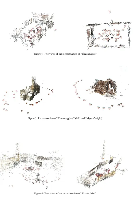
Figure 4: Two views of the reconstruction of “Piazza Dante”
Figure 5: Reconstruction of “Pozzoveggiani” (left) and “Myson” (right)
Figure 7: Two views of the reconstruction of “Piazza Bra”
Figure 8: Two views of the reconstruction of “St Jean Fountain”
Image set resolution images: notes orig/oriented
Pozzoveggiani 1024x768 50/54
Piazza Dante 2288x1712 39/39 half res Piazza Erbe 2288x1712 183/259 half res Piazza Bra 3008x2000 217/331
Castle-K19 3072x2048 19/19 Fountain-K6 3072x2048 6/6 Herz-Jesu-K7 3072x2048 7/7 Myson 3872x2592 18/18
StJean Fount.n 6048x4032 66/66 half res autocalibrated Piazza Navona 4000x3000 53/92 wrong Campidoglio 3000x4000 34/56 wrong Parc Guell 3000x4000 38/53 wrong
Table 2: Summary of results.
Future work will be aimed at bridging the “semantic web”, mov-ing from an unstructured cloud of points to a higher level model that can imported in any digital content creation software. Our first step in this direction is described in (Toldo and Fusiello, 2010).
Data and additional material are available from from http://profs.sci.univr.it/∼fusiello/demo/samantha/.
ACKNOWLEDGEMENTS
The use of VLFeat by A. Vedaldi and B. Fulkerson, ANN by David M. Mount and Sunil Arya, SBA by M. Lourakis and A. Ar-gyros is gratefully acknowledged. Images have been provided by F. Remondino (FBK, Trento) and Christof Strecha (EPFL, Lau-sanne). This work has been partly supported by the EU SAMU-RAI project (Grant No. 217899).
REFERENCES
Agarwal, S., Snavely, N., Simon, I., Seitz, S. M. and Szeliski, R., 2009. Building rome in a day. In: Proc. Int. Conf. Computer Vision, Kyoto, Japan.
Brown, M. and Lowe, D., 2003. Recognising panoramas. In: Proc. Int. Conf. Computer Vision, Vol. 2, pp. 1218–1225.
Brown, M. and Lowe, D. G., 2005. Unsupervised 3D object recogni-tion and reconstrucrecogni-tion in unordered datasets. In: Proc. Int. Conf. on 3D Digital Imaging and Modeling.
Chum, O., Pajdla, T. and Sturm, P., 2005. The geometric error for homo-graphies. Computer Vision and Image Understanding 97(1), pp. 86–102.
Cornelis, N., Leibe, B., Cornelis, K. and Gool, L. V., 2008. 3D urban scene modeling integrating recognition and reconstruction. International Journal of Computer Vision 78(2-3), pp. 121–141.
Duda, R. O. and Hart, P. E., 1973. Pattern Classification and Scene Anal-ysis. John Wiley and Sons, pp. 98–105.
Farenzena, M., Fusiello, A. and Gherardi, R., 2009. Structure-and-motion pipeline on a hierarchical cluster tree. In: IEEE Int. Workshop on 3-D Digital Imaging and Modeling, Kyoto, Japan.
Fiore, P. D., 2001. Efficient linear solution of exterior orientation. IEEE Transactions on Pattern Analysis and Machine Intelligence 23(2), pp. 140–148.
Fitzgibbon, A. W. and Zisserman, A., 1998. Automatic camera recovery for closed and open image sequencese. In: Proc. Europ. Conf. Computer Vision, pp. 311–326.
Garro, V. and Fusiello, A., 2010. Toward Wide-Area Camera Localization for Mixed Reality. Eurographics Association, pp. 117–122.
Gherardi, R. and Fusiello, A., 2010. Practical autocalibration. In: Proc. Europ. Conf. Computer Vision, Lecture Notes in Computer Science, Springer Berlin / Heidelberg, pp. 790–801.
Gherardi, R., Farenzena, M. and Fusiello, A., 2010. Improving the ef-ficiency of hierarchical structure-and-motion. In: Proc. Int. Conf. Com-puter Vision and Pattern Rec.
Gibson, S., Cook, J., Howard, T., Hubbold, R. and Oram, D., 2002. Accurate camera calibration for off-line, video-based augmented reality. Mixed and Augmented Reality, IEEE / ACM Int. Symp. on.
Hampel, F., Rousseeuw, P., Ronchetti, E. and Stahel, W., 1986. Robust Statistics: the Approach Based on Influence Functions. Wiley Series in probability and mathematical statistics, John Wiley & Sons.
Hartley, R. and Zisserman, A., 2003. Multiple View Geometry in Com-puter Vision. Cambridge University Press.
Hartley, R. I. and Sturm, P., 1997. Triangulation. Computer Vision and Image Understanding 68(2), pp. 146–157.
Irschara, A., Zach, C. and Bischof, H., 2007. Towards wiki-based dense city modeling. In: Proc. Int. Conf. Computer Vision, pp. 1–8.
Kamberov, G., Kamberova, G., Chum, O., Obdrzalek, S., Martinec, D., Kostkova, J., Pajdla, T., Matas, J. and Sara, R., 2006. 3D geometry from uncalibrated images. In: Proc. 2nd Int. Symp. on Visual Computing. Lowe, D. G., 2004. Distinctive image features from scale-invariant key-points. International Journal of Computer Vision 60(2), pp. 91–110. Luong, Q.-T. and Faugeras, O. D., 1996. The fundamental matrix: The-ory, algorithms, and stability analysis. International Journal of Computer Vision 17, pp. 43–75.
Mount, D. M. and Arya, S., 1996. Ann: A library for approximate nearest neighbor searching. In: http://www.cs.umd.edu/ mount/ANN/. Ni, K., Steedly, D. and Dellaert, F., 2007. Out-of-core bundle adjustment for large-scale 3D reconstruction. In: Proc. Int. Conf. Computer Vision, pp. 1–8.
Nist´er, D., 2000. Reconstruction from uncalibrated sequences with a hierarchy of trifocal tensors. In: Proc. Europ. Conf. Computer Vision, pp. 649–663.
Nister, D. and Stewenius, H., 2006. Scalable recognition with a vocab-ulary tree. In: Proc. Int. Conf. Computer Vision and Pattern Rec., IEEE Computer Society, Washington, DC, USA, pp. 2161–2168.
Philbin, J., Chum, O., Isard, M., Sivic, J. and Zisserman, A., 2007. Object retrieval with large vocabularies and fast spatial matching. In: Proc. Int. Conf. Computer Vision and Pattern Rec.
Pollefeys, M., Verbiest, F. and Gool, L. V., 2002. Surviving dominant planes in uncalibrated structure and motion recovery. In: Proc. Europ. Conf. Computer Vision, pp. 837–851.
Quack, T., Leibe, B. and Van Gool, L., 2008. World-scale mining of objects and events from community photo collections. In: Proc. Int. Conf. on Content-based Image and Video Retrieval, pp. 47–56.
Schaffalitzky, F. and Zisserman, A., 2002. Multi-view matching for un-ordered image sets, or ”how do I organize my holiday snaps?”. In: Proc. Europ. Conf. Computer Vision, pp. 414–431.
Shum, H.-Y., Ke, Q. and Zhang, Z., 1999. Efficient bundle adjustment with virtual key frames: A hierarchical approach to multi-frame structure from motion. In: Proc. Int. Conf. Computer Vision and Pattern Rec. Simon, I., Snavely, N. and Seitz, S. M., 2007. Scene summarization for online image collections. In: Proc. Int. Conf. Computer Vision. Sivic, J. and Zisserman, A., 2003. Video Google: A text retrieval ap-proach to object matching in videos. In: Proceedings Int. Conf. on Com-puter Vision, Vol. 2, pp. 1470–1477.
Snavely, N., Seitz, S. M. and Szeliski, R., 2006. Photo tourism: explor-ing photo collections in 3D. In: SIGGRAPH: Int. Conf. on Computer Graphics and Interactive Techniques, pp. 835–846.
Steedly, D., Essa, I. and Dellaert, F., 2003. Spectral partitioning for struc-ture from motion. In: Proc. Int. Conf. Computer Vision, pp. 649–663. Thorm¨ahlen, T., Broszio, H. and Weissenfeld, A., 2004. Keyframe selec-tion for camera moselec-tion and structure estimaselec-tion from multiple views. In: Proc. Europ. Conf. Computer Vision, pp. 523–535.
Toldo, R. and Fusiello, A., 2010. Photo-consistent planar patches from unstructured cloud of points. In: Proceedings of the European Conference on Computer Vision (ECCV 2010), Lecture Notes in Computer Science, Springer Berlin / Heidelberg, pp. 589–602.
Torr, P. H. S., 1997. An assessment of information criteria for motion model selection. Proc. Int. Conf. Computer Vision and Pattern Rec. pp. 47–53.
Torr, P. H. S. and Zisserman, A., 2000. MLESAC: A new robust estimator with application to estimating image geometry. Computer Vision and Image Understanding 78, pp. 2000.