Apress Beginning SQL Queries From Novice To Professional Apr 2008 ISBN 1590599438 pdf

(1)

THE EXPERT’S VOICE

®

_{IN DATABASES}

Beginning

SQL Queries

From Novice to Professional

Clare Churcher

(2)

(3)

Beginning SQL Queries

From Novice to Professional

■ ■ ■

(4)

All rights reserved. No part of this work may be reproduced or transmitted in any form or by any means, electronic or mechanical, including photocopying, recording, or by any information storage or retrieval system, without the prior written permission of the copyright owner and the publisher.

ISBN-13 (pbk): 978-1-59059-943-3 ISBN-10 (pbk): 1-59059-943-8

ISBN-13 (electronic): 978-1-4302-0550-0 ISBN-10 (electronic): 1-4302-0550-4

Printed and bound in the United States of America 9 8 7 6 5 4 3 2 1

Trademarked names may appear in this book. Rather than use a trademark symbol with every occurrence of a trademarked name, we use the names only in an editorial fashion and to the benefit of the trademark owner, with no intention of infringement of the trademark.

Lead Editor: Jonathan Gennick Technical Reviewer: Darl Kuhn

Editorial Board: Clay Andres, Steve Anglin, Ewan Buckingham, Tony Campbell, Gary Cornell, Jonathan Gennick, Matthew Moodie, Joseph Ottinger, Jeffrey Pepper, Frank Pohlmann, Ben Renow-Clarke, Dominic Shakeshaft, Matt Wade, Tom Welsh

Project Manager: Beth Christmas

Distributed to the book trade worldwide by Springer-Verlag New York, Inc., 233 Spring Street, 6th Floor, New York, NY 10013. Phone 1-800-SPRINGER, fax 201-348-4505, e-mail orders-ny@springer-sbm.com, or visit http://www.springeronline.com.

For information on translations, please contact Apress directly at 2855 Telegraph Avenue, Suite 600, Berkeley, CA 94705. Phone 510-549-5930, fax 510-549-5939, e-mail info@apress.com, or visit http:// www.apress.com.

Apress and friends of ED books may be purchased in bulk for academic, corporate, or promotional use. eBook versions and licenses are also available for most titles. For more information, reference our Special Bulk Sales–eBook Licensing web page at http://www.apress.com/info/bulksales.

(5)

(6)

(7)

v

Contents at a Glance

About the Author

. . . xiii

About the Technical Reviewer

. . . xv

Acknowledgments

. . . xvii

Introduction

. . . xix

■

CHAPTER 1 Relational Database Overview

. . . 1

■

CHAPTER 2 Simple Queries on One Table

. . . 17

■

CHAPTER 3 A First Look at Joins

. . . 41

■

CHAPTER 4 Nested Queries

. . . 61

■

CHAPTER 5 Self Joins

. . . 77

■

CHAPTER 6 More Than One Relationship Between Tables

. . . 95

■

CHAPTER 7 Set Operations

. . . 107

■

CHAPTER 8 Aggregate Operations

. . . 133

■

CHAPTER 9 Efficiency Considerations

. . . 153

■

CHAPTER 10 How to Approach a Query

. . . 169

■

CHAPTER 11 Common Problems

. . . 191

■

APPENDIX

Sample Database

. . . 209

(8)

(9)

(10)

viii _■C O N T E N T S

Misusing Select to Answer Questions with the Word “both”

. . . 38

(11)

(12)

x _■C O N T E N T S

■

CHAPTER 8 Aggregate Operations

. . . 133

Simple Aggregates

. . . 133

The COUNT Function

. . . 133

The AVG Function

. . . 136

Other Aggregate Functions

. . . 138

Grouping

. . . 139

Filtering the Result of an Aggregate Query

. . . 143

Using Aggregates to Perform Division Operations

. . . 145

Nested Queries and Aggregates

. . . 147

Summary

. . . 150

■

CHAPTER 9 Efficiency Considerations

. . . 153

Indexes

. . . 153

Types of Indexes

. . . 154

Indexes for Efficiently Ordering Output

. . . 157

Indexes and Joins

. . . 158

What Should We Index?

. . . 160

Query Optimizer

. . . 161

What Does the Query Optimizer Consider?

. . . 161

Does the Way We Express the Query Matter?

. . . 162

Summary

. . . 167

■

CHAPTER 10 How to Approach a Query

. . . 169

Understanding the Data

. . . 169

Determine the Relationships Between Tables

. . . 169

The Conceptual Model vs. the Implementation

. . . 171

What Tables Are Involved?

. . . 173

Look at Some Data Values

. . . 174

Big Picture Approach

. . . 174

Combine the Tables

. . . 175

Find the Subset of Rows

. . . 176

Retain the Appropriate Columns

. . . 177

(13)

(14)

xii _■C O N T E N T S

Common Symptoms

. . . 202

No Rows Are Returned

. . . 202

Rows Are Missing

. . . 203

More Rows Than There Should Be

. . . 205

Statistics or Aggregates Incorrect

. . . 207

The Order Is Wrong

. . . 207

Common Typos and Syntax Problems

. . . 207

Summary

. . . 208

■

APPENDIX

Sample Database

. . . 209

(15)

xiii

About the Author

(16)

(17)

xv

About the Technical Reviewer

(18)

(19)

xvii

Acknowledgments

E

xpecting your friends and family to put up with you writing a book is a tough call. Writing a second book the following year is really pushing their patience. So I am very indebted to my family and colleagues for putting up with me again. Special thanks to my two “first draft readers.” My husband, Neville Churcher, and my friend and colleague Theresa McLennan both gave me many valuable suggestions on the first attempts at every chapter, and always did it in Clare time (i.e., now!) and with very good grace. Thanks also to all my good friends in the Applied Computing Group at Lincoln University, especially Alan McKinnon for his advice on Chapter 9.

(20)

(21)

xix

Introduction

A

s a query language, SQL is really quite small and should be easy to learn. A few basic ideas and a handful of keywords allow you to tackle a huge range of queries. However, many users often find themselves completely stumped when faced with a particular problem. You may find yourself in that group. It isn’t really a great deal of help for someone to say, “This is how I would do it.” What you need is a variety of ways to get started on a tricky problem. Once you have made a start on a query, you need to be able to check, amend, and refine your solution until you have what you need.

Two-Pronged Approach

Throughout this book, I approach different types of queries from two directions. The two approaches have their roots in relational algebra and calculus. Don’t be alarmed though— I won’t be delving into any complex mathematics. However, understanding a question and developing an appropriate SQL query do require logical thinking and precise definitions. The relational algebra and calculus approaches are both useful ways to grasp the logic and precision that are required to get accurate results.

The first approach, which has its roots in relational algebra, looks at how tables need to be manipulated in order to retrieve the subset of data you require. I describe the different types of operations that you can perform on tables, including joins, intersections, selections, and so on, and explain how to decide which might help in particular situations. Once you under-stand what operations are needed, translating them into SQL is relatively straightforward.

The second approach is what I use when I just can’t figure out which operations will give me the required results. This approach, based on relational calculus, lets you describe what an expected row in your result might be like; that is, what conditions it must obey. By looking at the data, it is surprisingly easy to develop a semiformal description of what a “correct” retrieved row would be like (and, by implication, how you would recognize an “incorrect” row). Because SQL was originally based on relational calculus, translating this semiformal description into a working query is particularly straightforward.

(22)

xx _■I N T R O D U C T I O N

Who This Book Is For

This book is for anyone who has a well-designed relational database and needs to extract some information from it. You might have noticed in the previous sentence that the data-base must be “well designed.” I can’t overemphasize this point. If your datadata-base is badly designed, it will not be able to store accurate and consistent data, so the information your queries retrieve will always be prone to inaccuracies. If you are looking to design a database from scratch, you should read my first book, Beginning Database Design (Apress, 2007). The final chapter of this book outlines a few common design problems you are likely to come across and gives some advice about how to mitigate the impact or correct the problem.

For this book, you do not need any theoretical knowledge of relational theory, as I will explain the relevant issues as they come up. The first chapter gives a brief overview of relational database theory, but it will help if you have had some experience working with databases with a few or more tables.

Objective of This Book

In this book, you will be introduced to all the main techniques and keywords needed to create SQL queries. You will learn about joins, intersections, unions, differences, selection of rows, and projection of columns. You will see how to implement these ideas in different ways using simple and nested queries, and you will be introduced to a variety of aggregate functions and summary techniques. You can try out what you learn using the sample data provided through the Apress web page for this book (http://www.apress.com/book/view/ 1590599438). There you will find the Access database used for the examples in the book and some scripts to create the database on a number of other platforms.

(23)

1

■ ■ ■

C H A P T E R 1

Relational Database Overview

A

query is a way of retrieving some subset of information from a database. That informa-tion might be a single number such as a product price, a list of members with overdue subscriptions, or some sort of calculation such as the total amount of products sold in the past 12 months. Once we retrieve this subset of data, we might want to update the data-base records or include the information in some sort of report.

Before getting into the nuts and bolts of how to build queries, it is necessary to under-stand some of the ideas and terminology associated with relational databases. In particular, it is useful to have a way of depicting how a particular database is put together, that is, what data is being kept in what tables and how everything is interrelated.

It is imperative that any database has been designed to accurately represent the situa-tion it is dealing with. With all the fanciest SQL in the world, you are unlikely to be able to get accurate responses to queries if the underlying database design is faulty. If you are setting up a new database, you should refer to a design book1 before embarking on the project.

In this chapter, we will look at some of the basic ideas of data models and relational theory so we can get started on formulating queries in SQL. Later chapters will expand on these ideas, as required. You will also learn about two important ways to think about queries: relational algebra and relational calculus.

What Is a Relational Database?

In simple terms, a relational database is a set of tables.2_{Each table keeps information} about aspects of one thing, such as a customer, an order, a product, a team, or a tourna-ment. It is possible to set up constraints on the data in individual tables and also between tables. For example, when designing the database, we might specify that an order entered in the Order table must exist for a customer who exists in the Customer table. How the tables are interrelated can be usefully depicted with a data model.

1. For instance, you can refer to my other Apress book, Beginning Database Design: From Novice to Professional (Apress, 2007).

(24)

2 C H A P T E R 1 ■ R E L A T I O N A L D A T A B A S E O V E R V I E W

Introducing Data Models

A data model provides us with information about how the data items in the database are interrelated. In this book, I will use an example of a golf club that has members who belong to teams and enter tournaments. One convenient way to give an overview of the different tables in a database is by using the class diagram notation from the Unified Modeling Language (UML).3 In this section, we will look at how to interpret a class diagram.

A class is like a template for a set of things (or events, people, and so on) about which we want to keep similar data. For example, we might want to keep names and other details about the members of our golf club. Figure 1-1 shows the UML notation for a Member class. The name of the class is in the top panel, and the middle panel shows the attributes, or pieces of data, we want to keep about each member. Each member can have a value for LastName, FirstName, and so on.

Figure 1-1. UML representation of a Member class

Each class in a data model will be represented in a relational database as a table. The attributes are the columns (often referred to as fields) in the table, and the details of each member form the rows in the table. Figure 1-2 shows some example data.

The data model can also depict the way the different classes in our database depend on each other. Figure 1-3 shows two classes, Member and Team, and how they are related.

The pair of numbers at each end of the plays for line in Figure 1-3 indicates how many members play for one particular team, and vice versa. The first number of each pair is the minimum number. This is often 0 or 1 and is therefore sometimes known as the option-ality (that is, it indicates whether a member must have an associated team, or vice versa). The second number (known as the cardinality) is the greatest number of related objects. It is usually 1 or many (denoted by n or *), although other numbers are possible.

(25)

C H A P T E R 1 ■ R E L A T I O N A L D A T A B A S E O V E R V I E W 3

Figure 1-2. A table representing the instances of our Member class

Figure 1-3. A relationship between two classes

Relationships are read in both directions. Reading Figure 1-3 from left to right, we have that one particular member doesn’t have to play for a team and can play for at most one team (the numbers 0 and 1 at the end of the line nearest the Team class). Reading from right to left, we can say that one particular team doesn’t need to have any members and can have many (the numbers 0 and n nearest the Member class). A relationship like the one in Figure 1-3 is called a 1-Many relationship (a member can belong to just one team, and a team can have many members). Most relationships in a relational database will be 1-Many relationships.

For members of a team, you might think there should be exactly four members (say for an interclub team). Although this might be true when the team plays a round of golf, our database might record different numbers of members associated with the team as we add and remove players through the year. A data model usually uses 0, 1, and many to model the relationships between tables. Other constraints (such as the maximum number in a team) are more usually expressed with business rules or with UML use cases.4

(26)

Introducing Tables

The earlier description of a relational database as a set of tables was a little oversimplified. A more accurate definition is that a relational database is a set of relations. When people refer to tables in a relational database, they generally assume (whether they know it or not) that they are dealing with relations. The reason for the distinction between tables and relations is that there is a well-defined set of operations on relations that allow them to be combined and manipulated in various ways.5_{This is exactly what we need in order to be} able to extract accurate information from a database. We won’t be covering the actual mathematics in this book, but we will be using the operations. So, in nonmathematical speak, what is so special about relations?

One of the most important features of a relation is that it is a set of unique rows.6_No two rows in a relation can have identical values for every attribute. A table does not gener-ally have this restriction. If we consider our member data, it is clear why this uniqueness constraint is so important. If, in the table in Figure 1-2, we had two identical rows (say for Brenda Nolan), we would have no way to differentiate them. We might associate a team with one row and a subscription payment with the other, thereby generating all sorts of confusion.

The way that a relational database maintains the uniqueness of rows is by specifying a primary key. A primary key is an attribute, or set of attributes, that is guaranteed to be different in every row of a given relation. For data such as the member data in this example, we cannot guarantee that all our members will have different names or addresses (a dad and son may share a name and an address and both belong to the club). To help distin-guish different members, we have included an ID number as one of the member attributes, or fields. You will find that adding an identifying number (colloquially referred to as a surrogate key) is very common in database tables. If MemberID is defined as the primary key for the Member table, then the database system will ensure that in every row the value of MemberID is different. The system will also ensure that the primary key field always has a value. That is, we can never enter a row that has an empty MemberID field. These two requirements for a primary key field (uniqueness and not being empty) ensure that given the value of MemberID, we can always find a single row that represents that member. We will see that this is very important when we start establishing relationships between tables later in this chapter. Once a table has a primary key nominated, then it satisfies the uniqueness requirement of a relation.

Another feature of a relation is that each attribute (or column) has a domain. A domain is a set of allowed values and might be something very general. For example, the domain for the FirstName attribute in the Member table is just any string of characters, for example, “Michael” or “Helen.” The domain for columns storing dates might be any valid date (so that February 29 is allowed only in leap years), whereas for columns keeping quantities,

(27)

the domain might be integer values greater than 0. All database systems have built-in domains or types such as text, integer, or date that can be chosen for each of the fields in a table. Systems vary as to whether users can define their own more highly specified domains that they can use across different tables; however, all good database systems allow the designer to specify constraints on a particular attribute in a table. For example, in a partic-ular table we might specify that a birth date is a date in the past, that the value for a gender field must be “M” or “F”, or that a student’s exam mark is between 0 and 100. The idea of domains becomes important for queries when we need to compare values of columns in different tables.

When I refer to a database table in this book, I mean a set of rows with a nominated primary key to ensure every row is different and where every column has a domain of allowed values. Listing 1-1 shows the SQL code for creating the Member table with the attribute names and domains specified. In SQL, the keyword INT means an integer or nonfractional number, and CHAR(n) means a string of characters n long. The code also specifies that MemberID will be the primary key. (Listing 1-1 doesn’t create the relationship with the Team table yet.) The code is fairly self-explanatory.

Listing 1-1. SQL to Create the Member Table

CREATE TABLE Member (

Inserting and Updating Rows in a Table

The emphasis in this book is on getting accurate information out of a database, but the data has to get in somehow. Most database application developers will provide user-friendly interfaces for inserting data into the various tables. Often a form is presented to the user for entering data that may end up in several tables. Figure 1-4 shows a simple Microsoft Access form that allows a user to enter and amend data in the Member table.

(28)

Figure 1-4. A form allowing entry and updating of data in the Member table

Listing 1-2 shows the SQL to enter one complete row in our Member table. The data items are in the same order as specified when the table was created (Listing 1-1). Note that the date and string values need to be enclosed in single quotes.

Listing 1-2. Inserting a Complete Row into the Member Table

INSERT INTO Member

VALUES (118, 'McKenzie', 'Melissa', '963270', 30, '05/10/1999', 'F')

If many of the data items are empty, we can specify which attributes or fields will have values. If we had only the ID and last name of a member, we could insert just those two values as in Listing 1-3. Remember that we always have to provide a value for the primary key field.

Listing 1-3. Inserting a Row into the Member Table When Only Some Attributes Have Values

INSERT INTO Member (MemberID, LastName) VALUES (258, 'Olson')

(29)

Listing 1-4. Updating a Row in the Member Table

UPDATE Member SET Phone = '875077' WHERE MemberID = 118

Designing Appropriate Tables

Even a quite modest database system will have hundreds of attributes: names, dates, addresses, quantities, descriptions, ID numbers, and so on. These all have to find their way into tables, and getting them in the right tables is critical to the overall accuracy and usefulness of the database. Many problems can arise from having attributes in the wrong tables. As a simple illustration of what can go wrong, I’ll briefly show the problems associated with having redundant information.

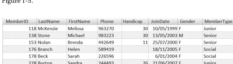
Say we want to add membership types and fees to the information we are keeping about members of our golf club. We could add these two fields to the Member table, as in Figure 1-5.

Figure 1-5. Possible Member table

If the fee for all senior members is the same (that is, there are no discounts or other complications), then immediately we can see there has been a problem with the data entry because Thomas Spence has a different fee from the other senior members. The piece of information about the fee for a senior member is being stored several times, so inevitably inconsistencies will arise. If we formulated a query to find the fee for seniors, what would we expect for an answer? Should it be $300, $280, or both?

(30)

The problem is that we are trying to keep information about two different things in our Member table: information about each member (IDs, names, and so on) and information about membership types (the different fees). This means the Fee attribute is in the wrong table. Figure 1-6 shows a better solution with two classes: one for information about members and one for information about membership types. The tables have a 1-Many relationship between them that can be read from left to right as “each member has one membership type” and in the other direction as “a particular membership type can have many associ-ated members.”

Figure 1-6. Separating members and their types

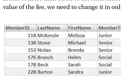
We can represent the model in Figure 1-6 with the two tables in Figure 1-7. (A few of the fields in the Member table have been hidden in Figure 1-7 just to keep the size manageable.) You can see that we have now avoided keeping the information about the fee for a senior member more than once, so inconsistencies do not arise. Also, if we need to change the value of the fee, we need to change it in only one place.

Figure 1-7. Member and Type tables

If we need to find out what fee Thomas Spence pays, we now need to consult two tables: the Member table to find his type and then the Type table to find the fee for that type. The bulk of this book is about how to do just that sort of data retrieval. We can formulate queries to accurately retrieve all sorts of information from several tables in the database.

(31)

At the risk of repeating myself, I do want to caution you about the necessity of ensuring that the database is properly designed. The simple model in Figure 1-6 is almost certainly quite unsuitable even for the tiny amount of data it contains. A real club will probably want to keep track of fees and how they change over the years. They may need to keep records of when members graduated from junior to senior. They may offer discounts for prompt payments. Designing a useful database is a tricky job and outside the scope of this book.7

Maintaining Consistency Between Tables

Even the smallest database will have many, many tables. We saw in the previous section that keeping just a tiny amount of data for members required two tables if it was to be accurately maintained. Database systems provide domains or other constraints to ensure that values in particular columns of a given table are sensible, but we can also set up constraints between tables.

Look at the modified data in Figure 1-8. What fee does Melissa McKenzie pay now?

Figure 1-8. Inconsistent data between tables

We can probably make an educated guess that Melissa is probably meant to be a “Junior” rather than a “Junor”, but we don’t want our database to be second-guessing what it thinks we mean. We can prevent typos like this by placing a constraint called a foreign key on the Member table. We tell the database that the MemberType column in the Member table can have only a value that already exists as a primary key value in the Type table (for this example, that means it must be either “Junior”, “Senior”, or “Social”). The terminology for this is to “create the MemberType field as a foreign key that references the Type table.” With this constraint in place, “Junior” is OK because we have a row in the Type

7. For more information about database design, refer to my other Apress book, Beginning Database Design: From Novice to Professional (Apress, 2007).

(32)

table with “Junior” in the primary key, but “Junor” will not be accepted. In general, all 1-Many relationships between classes in a data model are set up this way.

Listing 1-5 shows the SQL for creating the Member table with a foreign key constraint.

Listing 1-5. SQL to Create the Member Table with a Foreign Key

CREATE TABLE Member( MemberID INT PRIMARY KEY, LastName CHAR(20), FirstName CHAR(20), Phone CHAR(20), Handicap INT, JoinDate DATETIME, Gender CHAR(1),

MemberType CHAR(20) FOREIGN KEY REFERENCES Type)

Most database products also have graphical interfaces for setting up and displaying foreign key constraints. Figure 1-9 shows the interfaces for SQL Server and Access. These diagrams, which are essentially implementations of the data model, are invaluable for understanding the structure of the database so we know how to extract the information we require.

Figure 1-9. Diagrams for implementing 1-Many relationships using foreign keys

Retrieving Information from a Database

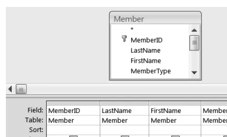
Now that we have the starting point of a well-designed database consisting of a set of interrelated, normalized tables, we can start to look at how to extract information by way of queries. Many database systems will have a diagrammatic interface that can be very useful for many simple queries. Figure 1-10 shows the Access interface for retrieving the names of senior members from the Member table. The check marks denote which columns we want to see, and the Criteria row enables us to specify particular rows.

(33)

Figure 1-10. Access interface for a simple query on the Member table

We can express the same query in SQL as shown in Listing 1-6. It contains three clauses: SELECT specifies which columns to return, FROM specifies the table(s) where the infor-mation is kept, and WHERE specifies the conditions the returned rows must satisfy. We’ll look at the structure of SQL statements in more detail later, but for now the intention of the query is pretty clear.

Listing 1-6. SQL to Retrieve the Names of Senior Members from the Member Table

SELECT FirstName, LastName FROM Member

WHERE MemberType = 'Senior'

These two methods of expressing a simple query are quite straightforward, but as we need to include more and more tables connected in a variety of ways, the diagrammatic interface rapidly becomes unwieldy and the SQL commands more complex.

Often, it is easier to think about a query in a more abstract way. With a clear abstract understanding of what is required, it then becomes more straightforward to turn the idea into an appropriate SQL statement. There are two different abstract ways to consider queries on a relational database. Because relational theory was developed by a mathematician, it is couched in quite mathematical terms. The two equivalent ways of thinking about queries are called relational algebra and relational calculus. Do not be alarmed! We will not be getting into quadratic equations or integration—I promise. However, these two methods might take a bit of getting used to, so treat the examples in this chapter as just a taster; we will be going over the details in later chapters.

Relational Algebra: Specifying the Operations

(34)

different ways of combining data from two tables. (Remember that when I talk about tables, I really mean ones with unique rows.) Every time we use one of the operations on a table, the result is another table. This means we can build up quite complicated queries by taking the result of one operation and applying another operation to it.

We will look at all the different operations in detail throughout the book, but just as a simple example we will discuss how to use relational algebra to retrieve the names of the senior members of our golf club. We will need two operations. The select operation returns just those rows from a table that satisfy a particular condition. The project operation returns just the specified columns.

First we’ll get just the rows we need. We can say it like this:

Apply the select operation to the Member table with the condition that the

MemberType field must have the value “Senior”.

Clearly, this is all going to get a bit wordy as we apply more and more operations, so it is useful to introduce some shorthand, as shown in Listing 1-7. σ (the Greek letter sigma) stands for the select operation, and the condition is specified in the subscript. For conve-nience I have called the resulting table SenMemb.

Listing 1-7. The Select Operation to Retrieve the Subset of Rows for Seniors

Figure 1-11 shows the result of this operation. Having retrieved a table with the appro-priate rows, we now apply the project operation to get the right columns. Listing 1-8 shows the shorthand for this, where π (pi) denotes the project operation and the columns are specified in the subscript.

Listing 1-8. The Project Operation to Retrieve a Subset of Columns

You can express the whole algebra expression in one go, as shown in Listing 1-9.

Listing 1-9. The Complete Algebra Expression

Figure 1-11 shows the original, intermediate, and final tables. Note that the interme-diate and final tables are not permanent in the database.

The example in Figure 1-11 shows how we can apply two relational algebra operations in succession to retrieve a final relation with the required data. We do not really need the power of the relational algebra to visualize how to formulate a query this simple; however, most queries are not this simple.

(35)

Figure 1-11. Result of two successive relational algebra operations

Relational Calculus: Specifying the Result

Relational algebra lets us specify a sequence of operations that eventually result in a set of rows with the information we require. As we will see throughout this book, there may be several different ways of applying a sequence of relational operations that will retrieve the same data. The other method that relational theory provides for describing a query is rela-tional calculus. Rather than specifying how to do the query, we describe what conditions the resulting data should satisfy. Once again, this may take a bit of getting used to, so we will go over all this more carefully in later chapters.

In nonformal language, a relational calculus description of a query has the following form:

I want the set of rows that obey the following conditions . . .

As with the algebra version, this can become very wordy, so shorthand is convenient, as shown in Listing 1-10.

Listing 1-10. General Form of a Query Expressed in Relational Calculus

{ m | condition(m) }

The part on the left of the bar will contain a description of the attributes or columns we want returned, while the part on the right describes the criteria they must satisfy. The letter m is a way of referring to a particular row (m) in a table, and we will need to intro-duce other labels when we have several tables to contend with. An example is the best way to clarify what a relational calculus expression means. Listing 1-11 shows the relational calculus for the query to retrieve senior club members.

Listing 1-11. Relational Calculus to Retrieve Senior Members

{m | Member(m) and m.MemberType = 'Senior'}

(36)

We can interpret Listing 1-11 like this:

Retrieve each row (m) from the Member table where the MemberType attribute of that row has the value “Senior”.

We can further refine the query as in Listing 1-12, which retrieves just the names of the senior members.

Listing 1-12. Relational Calculus to Retrieve the Names of Senior Members

{m.LastName, m.FirstName | Member(m) and m.MemberType = 'Senior'}

We can interpret Listing 1-12 like this:

Retrieve the values of the FirstName and LastName attributes from all the rows m where m comes from the Member table and the MemberType attribute of those rows has the value “Senior”.

Why are we doing this? Admittedly, it is over the top to introduce this notation for such a simple query, but as our queries become more complex and involve several tables, it is useful to have a way to express the criteria in an unambiguous way. Also, SQL is based on relational calculus. In Listing 1-12 if you replace the bar (|) with the SQL keyword FROM and the “and” with the keyword WHERE, then you essentially have the SQL query of Listing 1-6.

Why Do We Need Both Algebra and Calculus?

It would be reasonable to also ask, why do we need either? As mentioned earlier, we do not need these abstract ideas for simple queries. However, if all queries were simple, you would not be reading this book. In the first instance, queries are expressed in everyday language that is often ambiguous. Try this simple expression: “Find me all students who are younger than 20 or live at home and get an allowance.” This can mean different things depending on where you insert commas. Even after we have sorted out what the natural-language expression means, we then have to think about the query in terms of the actual tables in the database. This means having to be quite specific in how we express the query. Both relational algebra and relational calculus give us a powerful way of being accurate and specific.

(37)

to explicitly specify algebraic operations such as joins, products, and unions on the tables as well.

There are often several equivalent ways of expressing an SQL statement. Some ways are very much based on calculus, some are based on algebra, and some are a bit of both. I have been teaching queries to university students for several years. For some complicated queries, I often ask the class whether they find the calculus or algebra expressions more intuitive. The class is usually equally divided. Personally I find some queries just feel obvious in terms of relational algebra, whereas others feel much more simple expressed in rela-tional calculus. Once I have the idea pinned down with one or the other, the translation into SQL (or some other query language) is usually straightforward.

The more tools you have at your disposal, the more likely you will be able to express complex queries accurately.

Summary

This chapter has presented an overview of relational databases. We have seen that a rela-tional database consists of a set of tables that represent the different aspects of our data (for example, a table for members and a table for types). Each table has a primary key that is a field(s) that is guaranteed to have a different value for every row, and each field (or column) of the table has a set of allowed values (a domain).

We have also seen that it is possible to set up relationships between tables with foreign keys. A foreign key is a value in one table that has to already exist as the primary key in another table. For example, the value of MemberType in the Member table must be one of the values in the primary key field of the Type table.

It is often helpful to think about queries in an abstract way, and there are two ways to do this. Relational algebra is a set of operations that can be applied to tables in a database. It is a way of describing how we need to manipulate the tables to extract the information we require. Relational calculus is a way of describing what criteria our required informa-tion must satisfy.

(38)

(39)

17

■ ■ ■

C H A P T E R 2

Simple Queries on One Table

I

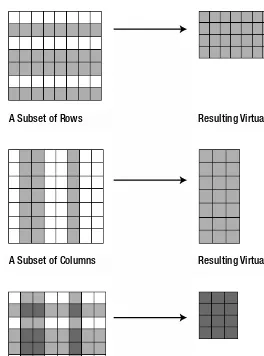
f a database has been designed correctly, the data will be in several different tables. For example, our golf database is likely to have separate tables for information about members, teams, and tournaments, as well as tables that connect these values, for example, which members play in which teams, enter which tournaments, and so on. To make the best use of our data, we will need to combine values from different tables. As we work through complicated combinations, we can imagine the set of rows resulting from each step being put into a “virtual” table. We can think of a virtual table as one that is made to order and is only temporary. At each step we may be interested in only some of the data in the virtual table. In this chapter, we will look at choosing values from just one table. The table may be one of the permanent tables in our database, or it may be a virtual table that has been temporarily put together as part of a more complicated query.

(40)

18 C H A P T E R 2 ■ S I M P L E Q U E R I E S O N O N E T A B L E

Figure 2-1. Retrieving subsets of rows and columns from a single table

Simple queries like this can provide information for reports, subsets of data for anal-ysis, and answers to specific questions. Figure 2-2 shows some examples for the Member table from our golf club database.

A Subset of Rows Resulting Virtual Table

A Subset of Columns Resulting Virtual Table

(41)

C H A P T E R 2 ■ S I M P L E Q U E R I E S O N O N E T A B L E 19

Figure 2-2. Examples of simple queries on the Member table

Retrieving rows and columns uses the relational algebra operations select and project. Nearly all queries will at some stage include the select and project operations.

a) Subset of rows: All the information about men

b) Subset of columns: Phone list for all members

c) Subset of both rows and columns: Handicaps for Junior members

(42)

Retrieving a Subset of Rows

Retrieving a subset of rows is one of the most common operations we will carry out in a query. In the following sections, we will look at retrieving rows from one of the original tables in our database. The same ideas apply to selecting rows from virtual tables resulting from other manipulations of our data.

Relational Algebra for Retrieving Rows

The relational algebra select operation retrieves rows from a table. To decide which rows to retrieve, we need to specify a condition for the operation. Basically, a condition is a statement that is either true or false. We apply the condition to each row in the table inde-pendently, retaining those rows for which the condition is true and discarding the others. Say we want to find all the men our club, as in Figure 2-2a. Fortunately, when we designed our database in Chapter 1, we foresaw such a query and included an attribute Gender in the Member table. We want just that subset of rows where the value in the Gender field is “M”, so this becomes the condition for the select operation.

Listing 2-1 shows the notation for this operation. The Greek letter sigma (σ) is short-hand for select, the table we are applying the operation to is in parentheses (Member), and the subscript Gender = 'M' is the condition.

Listing 2-1. The Select Operation to Retrieve All the Men from the Member Table

What if we want to find everyone with a handicap under 12? This will again be a subset of rows from the Member table, so the select operation will do the trick. The condition this time depends on the value in the Handicap column. We want any rows where the value of Handicap is less than 12. Listing 2-2 shows the relational algebra for retrieving the required rows. We will look more closely at how to express more complex conditions in the next section.

Listing 2-2. The Select Operation Used to Retrieve Members with Handicaps Under 12

Relational Calculus for Retrieving Rows

The relational algebra describes how we should retrieve the required information from our database; in the previous cases, it’s by saying “Go and get the subset of rows that satisfy this condition.” The relational calculus describes what the required information is like.

(Member)

σGender='M'

(Member)

(43)

Listing 2-3 shows the shorthand for expressing the calculus for retrieving men from the Member table.

Listing 2-3. The Calculus Expression to Retrieve All the Men from the Member Table

{m | Member(m) and m.Gender = 'M'}

The part on the right of the vertical bar (|) is the description of the retrieved rows. The expression in Listing 2-3 can be interpreted as saying “I want a set of rows that come from the Member table, and each row must have ‘M’ as the value for the Gender attribute.”

The letter m in Listing 2-3 is officially called a tuple variable, but I’ll refer to it as a row variable (which is not strictly accurate but a bit easier to understand). I like to think of the variable acting like a finger, as in Figure 2-3. The finger (labeled m) points to each row in the Member table and checks to see whether it obeys the condition that its Gender attribute has the value “M”. As our queries get more complex, we will have many different fingers pointing at different tables.

Figure 2-3. Row variable m investigating each row of the Member table

SQL for Retrieving Rows

Listing 2-4 shows the SQL statement for retrieving information about the men in our golf club.

Listing 2-4. The SQL Statement to Retrieve All the Men from the Member Table

SELECT * FROM Member WHERE Gender = 'M'

This query has three parts, or clauses: The SELECT1 clause says what information to retrieve. In this case, * means retrieve all the columns. The FROM clause says which table(s)

1. Note that in SQL the keyword SELECT just means that a given statement is a query for retrieving infor-mation. It doesn’t mean that the statement is necessarily going to involve an algebra select operation.

(44)

the query involves, and the WHERE clause describes the condition for deciding whether a particular row should be included in the result. Our condition says to check the value in the field Gender. In SQL when we specify an actual value for a character field, we need to enclose the value in single quotes, as in 'M'.

Retrieving a Subset of Columns

Now let’s look at how we can specify that we want to see only some of the columns in our result, perhaps just names and phone numbers as in Figure 2-2b. Once again, this is an operation that we can apply to an original table in our database or to a virtual table resulting from some complex combination of several tables.

Relational Algebra for Retrieving Columns

The relational algebra operation for retrieving a subset of columns is project, and we represent it with the Greek letter pi (π). Listing 2-5 shows the algebra for selecting the names and phone numbers from our Member table.

Listing 2-5. The Project Operation to Retrieve Names and Phone Numbers from the Member Table

The columns we want to retrieve (LastName, FirstName, and Phone) are specified in the subscript.

Relational Calculus for Retrieving Columns

Our notation for expressing a calculus query is in two parts separated by a bar, as in Listing 2-6. The part on the left describes what information we want to retrieve (in this case the LastName, FirstName, and Phone columns), and the part on the right describes the condition. In this case, the condition is only that the row comes from the Member table because we want the information for all our members.

Listing 2-6. The Calculus Expression to Retrieve Names and Phone Numbers from the Member Table

{m.LastName, m.FirstName, m.Phone | Member(m) }

Once again, it is useful to think of the row variable m as being a finger pointing at each row, deciding whether it is to be included and then retrieving the specified attributes of that row.

(Member)

(45)

SQL for Retrieving Columns

We specify what columns we want to retrieve in the SELECT clause of an SQL query. Whereas previously we used * to say “return all the columns,” Listing 2-7 now specifies the subset of columns we want in our result.

Listing 2-7. The SQL for Retrieving Names and Phone Numbers from the Member Table

SELECT LastName, FirstName, Phone FROM Member

Because we want to see all these column values for every row, this query doesn’t need a WHERE clause.

Using Aliases

The query in Listing 2-7 works just fine, but as our queries get more complicated and involved, we will have a number of different tables. Some of the tables may have the same column names, and we might need to distinguish them. Therefore, we can preface each of the attributes in our query with the name of the table that they come from, as in Listing 2-8.

Listing 2-8. Prefacing Attribute Names with the Table Name

SELECT Member.LastName, Member.FirstName, Member.Phone FROM Member

Because typing the whole table name can become tiresome and also because in some queries we might need to compare data in more than one row of a table, SQL has the notion of an alias. Have a look at Listing 2-9.

Listing 2-9. Using an Alias

SELECT m.LastName, m.FirstName, m.Phone FROM Member m

In the FROM clause, we have declared an alias or alternative name for the Member table, in this case m. We can give our alias any name or letter we like; short is good. Then in the rest of the query we can use the alias whenever we want to specify an attribute from that table.

(46)

Combining Subsets of Rows and Columns

In the previous sections, we saw the algebra operations select (a subset of rows) and project (a subset of columns) acting independently. One of the most powerful features of the algebra is that the result of an operation is another table (or, more formally, another set of unique rows). This means we can apply another operation to the result of the first operation and so build up complex queries.

We can use successive operations to create an algebra expression for the query in Figure 2-2c, retrieving the names and handicaps of junior members. First we find the rows for juniors using a select operation, and then we use a project operation to retrieve the required columns from the result. Listing 2-10 shows the full expression.

Listing 2-10. Combining a Select and Project Operation

π_{LastName, FirstName, Handicap} (σ_{MemberType = 'Junior'} (Member))

As you can see, the algebra tells us how to get the result we want. First get the appro-priate rows, and then get the required columns. The calculus doesn’t tell us how to carry out a series of steps; it just describes what the final set of rows will be like. Have a look at Listing 2-11.

Listing 2-11. Calculus Expression to Retrieve Handicaps of Junior Members

{m.Lastname, m.FirstName, m.Handicap | Member(m) and m.MemberType = 'Junior'}

The left side of the expression in Listing 2-11 says we are going to retrieve the LastName, FirstName, and Handicap values from some row m. The right side of the expression tells us which rows to include. Picture a finger labeled m, as in Figure 2-3. The expression in Listing 2-11 says that our finger m is going to scan rows in the Member table and include those rows where the value of MemberType is “Junior”.

Now look at Listing 2-12, which shows the SQL for this query.

Listing 2-12. SQL Statement to Retrieve Handicaps of Junior Members

SELECT m.Lastname, m.FirstName, m.Handicap FROM Member m

WHERE m.MemberType = 'Junior'

(47)

Saving Queries

I’ve been talking in a rather imprecise manner about “retrieving” rows and “returning” information. What happens to the rows that result from a query? In reality, we are not getting information and putting it anywhere; we are just looking at a subset of the infor-mation in the tables in our database. If the data in the underlying database changes, then the results of our query will change too. A query is like a window on our database through which we can see just the information we require. It doesn’t hurt to think about the infor-mation that results from a query being in the form of a “virtual” table as long as you realize it is just temporary. The images in Figure 2-2 are results of queries, but they are not real tables—just different windows into the underlying Member table.

It is possible to keep the result of a query in a new permanent table (sometimes called a snapshot), but we usually don’t want to do that because it will become out of date if the underlying data changes. What we usually want to do is save the instructions so that we can ask the same question another day. Consider our phone list query. Every so often after the membership of the club has been updated, we might want to see a new phone list. Rather than having to write the query in Listing 2-7 each time, we can save the instructions in what is known as a view. Listing 2-13 shows how we can create a view so we can see up-to-date phone lists. We have to give the view a name, which can be anything we want (PhoneList seems sensible), and then we supply the SQL statement (as in Listing 2-7) for retrieving the appropriate data.

Listing 2-13. Creating a View So You Can Use the Same Query Many Times

CREATE VIEW PhoneList AS

SELECT m.LastName, m.FirstName, m.Phone FROM Member m

PhoneList now becomes a “virtual” table, and we can use it like one of our real tables in other queries. We just need to remember that the virtual table is created on the fly by running the query on the permanent Member table and is then gone. To get our phone list now, we can use the SQL statement in Listing 2-14.

Listing 2-14. Using a View in a Query

SELECT * FROM PhoneList

Specifying Conditions for Selecting Rows

(48)

value in just one field, such as MemberType = 'Junior'. In the following section, we will look more closely at the different ways you can specify quite complicated conditions.

Comparison Operators

A condition is a statement or expression that is either true or false, such as MemberType = 'Junior'. These types of expressions are called Boolean expressions after the 19th-century English mathematician George Boole who investigated their properties. The conditions we use to select rows from a table usually involve comparing the values of an attribute to some constant value. For example, we can ask whether the value of an attribute is the same, different, or greater than some value. Table 2-1 shows some comparison operators we can use in our queries.

Just a quick note of caution. In Table 2-1, some of our examples compare numbers, and some compare text. When we compare text attributes, the comparison is alphabetical. “A” comes before “Z”, so “A” < “Z”. Similarly, “Ann” comes before “Azaria” alphabetically, so “Ann” < “Azaria,” and so on. Recall from Chapter 1 that when we create a table, we specify the type of each field; for example, MemberID was an INT (integer or whole number), and LastName was CHAR(20) (a 20-character field). With numeric fields like INT, comparisons are numerical. With text or character fields, comparisons are alphabetical, and with date and time fields, comparisons are chronological. If we put numbers in a character field, they will sort alphabetically. This means you have things like “40” < “5” (because the first char-acter, “4”, in the left text is less than the first charchar-acter, “5”, on the right side2_{). So, make} sure if a field in your table is going to contain numbers that you make it a numeric type, or you might get some rather surprising results from your queries.

Table 2-1. Comparison Operators

Operator Meaning Examples of True Statement

= Equals 5=5, 'Junior' = 'Junior' < Less than 4<5, 'Ann' < 'Zebedee' <= Less than or equal 4<=5, 5<=5

> Greater than 5>4, 'Zebedee' > 'Ann' >= Greater than or equal 5>=4, 5>=5

<> Not equal 5<>4, 'Junior' <> 'Senior'

(49)

With these comparison operators, we can create many different queries. Often we will compare a value of an attribute (say MemberType) to a literal value (say “Junior”). Table 2-2 shows some examples of Boolean expressions that we can use as conditions in the WHERE clause of an SQL statement for selecting rows from the Member table.

Some implementations of SQL are case sensitive when comparing text, and others are not. Being case sensitive means that, in comparisons, the different cases of the letters will make a difference; in other words, “Junior” is different from “junior”, which is different from “JUNIOR”. I usually check out any new database system I use to see what it does. If you do not care about the case of the attribute you are considering (that is, you are happy to retrieve rows where MemberType is “Junior” or “jUnIoR” or whatever), you can use the SQL function UPPER as in Listing 2-15. This will turn the value of each text attribute into uppercase before you do the comparison so that you know what is happening.

Listing 2-15. Selecting Rows Where the Case of a Text Value Is Not Important

SELECT * FROM Member m

WHERE UPPER(m.MemberType) = 'JUNIOR'

Logical Operators

We can also combine Boolean expressions to create more interesting conditions. For example, we can specify that two expressions must both be true before we retrieve a particular row.

Let’s assume we want to find all the junior girls. This requires two conditions to be true: they must be female, and they must be juniors. We can easily express each of these condi-tions independently. After that, we can use the logical operator AND, as in Listing 2-16, to say that both conditions must be true.

Table 2-2. Examples of Boolean Expressions on the Member Table

Expression Retrieved Rows

MemberType = 'Junior' All junior members

Handicap <= 12 All members with a handicap of 12 or less

JoinDate < '01/01/2000' Everyone who has been a member since before the beginning of 2000

(50)

Listing 2-16. Finding All the Junior Girls

WHERE m.MemberType = 'Junior' AND m.Gender = 'F'

Here we will look at three logical operators: AND, OR, and NOT. We have already seen how AND works. If we use OR between two expressions, then we require only one of the expressions to be true (but if they are both true, that is OK as well). NOT is used before an expression. For example, for our Member table, we might ask for rows obeying the condition NOT (MemberType = 'Social'). This means check each row, and if the value of MemberType is “Social”, then we don’t want that row. Table 2-3 gives some examples for the Member table. In the diagrams, each circle represents a set of rows (that is, those for social members or those for members with handicaps under 12). The shaded area represents the result of the operation.

Table 2-3. Examples of Logical Operators

Expression Description of Retrieved Data Diagram of Retrieved Data

MemberType = 'Senior' AND Handicap < 12

Seniors with a handicap under 12

MemberType = 'Senior' OR Handicap < 12

All the senior members as well as anyone else with a good handicap (those less than 12)

NOT MemberType = 'Social' All the members except the social ones (for the current data, that would be just the seniors and juniors)

Senior <12

(51)

The little truth tables in Figure 2-4 can be helpful in understanding and remembering how the Boolean operators work. You read them like this: In Figures 2-4a and 2-4b, we have two expressions, one along the top and one down the left. Each expression can have one of two values: True (T) or False (F). If we combine them with the Boolean expression AND, then Figure 2-4a shows that the overall statement is True only if both the contrib-uting statements are True (the square in the top left). If we combine them with an OR statement, then the overall statement is False only if both contributing statements are False (bottom right of Figure 2-4b). The table in Figure 2-4c says that if our original state-ment is True and we put NOT in front, then the result is False (left column), and vice versa.

Figure 2-4. Truth tables for logical operators (T = True, F = False)

Sometimes it can be a bit tricky turning natural-language descriptions into Boolean expressions. If you were asked for a list that included all the woman and all the juniors (don’t ask why!), you might translate this literally and write the condition MemberType = 'Junior' AND Gender = 'F'. However, the AND means both conditions must be true, so this would give us junior women. What our natural-language statement really means is “I want the row for any member if they are either a woman OR they are a junior (or both).” Be careful.

Dealing with Nulls

(52)

Figure 2-5. Table with missing data

When there is no value in a cell in a table, it is said to be Null. Nulls can cause a few headaches in a database. For example, if we ran two queries, one to produce a list of male members and the other a list of females, we might assume that all the members of the club would appear on one list or the other. However, for the data in Figure 2-5, we would miss Kim Jones. Now, you could argue that the data shouldn’t be like that—but we are talking about real people and real clubs with less than accurate and complete data. Maybe Kim forgot (or refused) to fill in the gender part of the application form. It is possible to insist that Nulls are not allowed in a field when we create a table. Listing 2-17 shows how we could make Gender a field that always requires a value.

Listing 2-17. SQL for Creating a Table with a Required Field

CREATE TABLE Member ( MemberID INT PRIMARY KEY, ...

Gender CHAR(1) NOT NULL,

...)

It is worth bearing in mind, however, that making fields required can create more head-aches than it cures. If Kim Jones did not fill all the boxes on his/her membership application but sent a bank draft for the subscription, then we want to make him/her a member and worry about the full details later. However, if we make Gender a required field, then we can’t enter a record for him/her in the table—or we have to guess what his/her gender is. Neither of these options is very good, so it is best to be sparing about making fields required. Remember that our primary key fields (by definition) always need a value.

(53)

Comparing Null Values

Given that we are going to have unexpected Nulls in our tables, it is important to know how to deal with them. What rows will match the two conditions in Listing 2-18?

Listing 2-18. What Rows Will Match Each of These Conditions

Gender = 'F' NOT (Gender = 'F')

If we run two queries with the conditions in Listing 2-18, will we get all the rows in the table? You might think that if we get all the rows that match a condition and all the ones that don’t, then we will get the lot. But in fact we don’t. Kim will not be included with the first condition because clearly the value of Gender does not equal “F”, But when we ask whether the value is NOT (“F”), we can’t say because we don’t know what the value is. It might be “F” if it had a value. This probably makes more sense if we think about handicaps. If we ask for everyone with Handicap > 12, NOT (Handicap > 12), or Handicap <=12, then Sarah’s row will never be retrieved because the question doesn’t apply to her—she doesn’t have a handicap.

So once we take Nulls into consideration, our expressions for conditions might actually have one of three values: True, False, or “don’t know.” That is pretty much how the world actually works if you think about it. Only rows that are True for a condition are retrieved in a query. If the condition is False or if we “don’t know,” then the row is not retrieved.

The truth tables, when we include “don’t know,”look like those in Figure 2-6. For an AND operation, if one expression is False, then it doesn’t matter about the others—the result will be False. For an OR operation, if one expression is True, then it doesn’t matter about the others, so the result will be True.

Figure 2-6. Truth tables with three valued logic ( T = True, F= False, ? = Don’t know)

(54)

Finding Nulls

Given that in our tables we may have Nulls that might cause us problems, it is useful to be able to find them. After we have entered a lot of new members into our database, we should check for problems. We might want to get a list of all the members who don’t have a value for MemberType, say. The SQL phrase to do this is IS NULL, as in Listing 2-19.

Listing 2-19. Finding the Members with No Value for MemberType

WHERE m.MemberType IS NULL

Alternatively, we might want to retrieve just those members who do have a value in a cell. If we wanted the names and handicaps of those members who have a value for Handicap, we could use the NOT operator to write a query like that in Listing 2-20.

Listing 2-20. Retrieving Information About Members Who Have a Handicap

WHERE NOT (m.Handicap IS NULL)

Managing Duplicates

Let’s get a little more formal for a moment. In Chapter 1, I explained that relational theory is based on mathematics and one of its main premises is that we are working with relations. A relation is a set of distinct rows. The fact that all the rows are different is important. Not only would it make no sense to have two identical rows about one of our members, but it would also get us into all sorts of trouble. I’ve been using the term table rather than relation but on the understanding that all our tables have a primary key, which ensures they meet the requirement that the rows are unique. When we use a project operation to retrieve a subset of columns, we may no longer have that primary key field in the result. Relational algebra depends on the result of each operation being another relation, and this is why it is possible to build up a series of operations to create quite complex queries. What do we do about possible duplicates? Let’s look at an example.

(55)

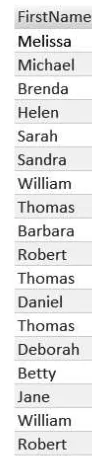
Figure 2-7. Projecting the FirstName column from the Member table

From a mathematical perspective, there is no question that in terms of the relational algebra the project operation will give us Figure 2-7b, a set of unique rows with the dupli-cates for William and Thomas removed. What would you have expected? It is useful to think about why we might carry out a query retrieving just names. Perhaps the query is to help prepare a set of nametags for a club party. If that is the case, then two Thomases and a William are going to feel a bit left out if we use the unique output.

For the previous example you might think, what’s all the fuss? Of course we want to keep all the rows. But let’s look at a different project operation to retrieve a list of member-ship types. Figure 2-8 shows the outputs with duplicates included and removed.

It’s pretty difficult to think of a situation where you want the duplicated rows in Figure 2-8a. The two project operations we have considered sound similar in natural language. “Give me a list of first names” and “Give me a list of membership types” sound like the same sort of question, but they mean something quite different. The first means “Give me a name for each member,” and the other means “Give me a list of unique membership types.”

(56)

Figure 2-8. Projecting the MemberType column from the Member table

What does SQL do? If we say SELECT MemberType FROM Member, we will get the output in Figure 2-8a with all the duplicates included. If we do not want the duplicates, then we can use the keyword DISTINCT, as in Listing 2-21.

Listing 2-21. Retrieving a List of Unique Membership Types

SELECT DISTINCT m.MemberType FROM Member m

Whether you keep the duplicates depends very much on the information you require, so you need to give it some careful thought. If you were expecting the set of rows in Figure 2-8b and got Figure 2-8a, you would most likely notice. With the two sets of rows in Figure 2-7, it is much more difficult to spot that you have perhaps made a mistake. Get into the habit of thinking about duplicates for all your queries.