CLASSIFICATION OF INFORMAL SETTLEMENTS THROUGH THE INTEGRATION
OF 2D AND 3D FEATURES EXTRACTED FROM UAV DATA
C.M. Gevaert a*, C. Persello a, R. Sliuzas a, G. Vosselman a
a Dept. of Earth Observation Science, ITC, University of Twente, Enschede, The Netherlands -
c.m.gevaert, c.persello, r.sliuzas, [email protected]
Commission III, WG III/4
KEY WORDS: informal settlements, image classification, point cloud, aerial imagery, Unmanned Aerial Vehicles (UAV), feature extraction, support vector machine
ABSTRACT:
Unmanned Aerial Vehicles (UAVs) are capable of providing very high resolution and up-to-date information to support informal settlement upgrading projects. In order to provide accurate basemaps, urban scene understanding through the identification and classification of buildings and terrain is imperative. However, common characteristics of informal settlements such as small, irregular buildings with heterogeneous roof material and large presence of clutter challenge state-of-the-art algorithms. Especially the dense buildings and steeply sloped terrain cause difficulties in identifying elevated objects. This work investigates how 2D radiometric and textural features, 2.5D topographic features, and 3D geometric features obtained from UAV imagery can be integrated to obtain a high classification accuracy in challenging classification problems for the analysis of informal settlements. It compares the utility of pixel-based and segment-pixel-based features obtained from an orthomosaic and DSM with point-pixel-based and segment-pixel-based features extracted from the point cloud to classify an unplanned settlement in Kigali, Rwanda. Findings show that the integration of 2D and 3D features leads to higher classification accuracies.
1. INTRODUCTION
Informal settlements are a growing phenomenon in many developing countries and the effort to promote the standard of living in these areas will be a key challenge for the urban planners of many cities in the 21st century (Barry and Rüther, 2005). The planning and execution of informal settlement upgrading projects require up-to-date base maps which accurately describe the local situation (UN-Habitat, 2012). For example, the identification of buildings gives an indication of the population in the area, classifying terrain identifies footpaths for accessibility and utility planning or free space for the location of infrastructure. However, such basic information is often lacking at the outset of upgrading projects (Pugalis et al., 2014), thus hindering the amelioration of the impoverished conditions in these areas. To create such base maps, satellite imagery is a powerful source of information regarding the physical characteristics of an informal settlement (Taubenböck and Kraff, 2013). However, as slums are often characterized by high building densities, small irregular buildings, and narrow footpaths, the spatial resolution provided by sub-meter satellite imagery is usually not sufficient (Kuffer et al., 2014). To this end, Unmanned Aerial Vehicles (UAVs) are useful as they can acquire imagery in a very flexible manner, and provide a cheap alternative to manned aerial surveys in order to generate orthomosaics with sub-decimeter resolution. Furthermore, UAV imagery can provide different data products like: a 2D orthomosaic, a 2.5D Digital Surface Model (DSM), and a 3D point cloud, resulting in a convenient alternative to the combined use of aerial images and LiDAR data. The question is: how to optimally integrate features from these datasets and assess their relative importance in order to accurately classify informal settlements to support upgrading projects?
The provision of 3D data is an important advantage of UAVs, as the inclusion of height information has been shown to greatly increase classification accuracy of urban scenes (Hartfield et al.,
* Corresponding author
2011; Longbotham et al., 2012; Priestnall et al., 2000). Especially the extraction of a normalized DSM (nDSM), which gives the elevation of pixels above the terrain, is useful for identifying elevated objects in urban scenes (Weidner and Förstner, 1995) and distinguishing between low vegetation and high vegetation (Huang et al., 2008). A recent overview of building detection methods based on aerial imagery and Airborne Laser Scanning (ALS) data indicates that state-of-the-art techniques which have access to both imagery and height information can identify large buildings with a very high correctness and completeness (Rottensteiner et al., 2014). However, these building detection algorithms face difficulties when the buildings are relatively small (i.e. less than 50m²), or when the height of the terrain is not uniform on all sides of the building due to sloped terrain. Unfortunately, informal settlements are often characterized by these challenging conditions, which emphasizes the need to investigate the synergies between 2D and 3D features to fully exploit the available UAV data and obtain a high classification accuracy.
calculate: the number of points within each bin, maximum height difference and standard deviation of height difference within each cell. Serna and Marcotegui (2014) use elevation maps to define the: minimum elevation, maximum elevation, elevation difference, and number of points per bin as a basis for detecting, segmenting and classifying urban objects. However, this method assumes the ground is planar. Guo et al. (2011) combined geometrical LiDAR features and multispectral features from orthoimagery to analyse which features were most relevant to classify an urban scene into: building, vegetation, artificial ground, and natural ground. They use elevation images to include the inclination angle and residuals of a local plane, but found that the maximum height difference between a LiDAR point and all other points within a specified radius was the most relevant feature.
There are two main limitations of the previous methods. Firstly, most methods explicitly or inherently assume the terrain to be planar. Attributes such as the maximum absolute elevation or height above the minimum point within a horizontal radius, which are often considered to be the most relevant features (Guo et al., 2011; Yan et al., 2015) will not serve to distinguish between buildings and terrain in a settlement located on a steep slope. Secondly, the methods generally focus on pixel-based features, or local neighbourhood features. However, Vosselman (2013) and Xu et al. (2014) indicate that segment-based point cloud features provide important supplementary information to pixel-based attributes. Similarly, Myint et al. (2011) found that 2D object-based attributes significantly improve the classification of urban scenes from VHR satellite imagery. Studies investigating the importance of features for urban scene classification should therefore consider segment-based features as well as point-based features.
The objective of this paper is to integrate the different information sources (i.e. UAV point cloud, DSM, and orthomosaic) and to analyse which 2D, 2.5D, and 3D feature sets are most useful for classifying informal settlements, a setting which challenges the boundaries of existing building detection algorithms. Feature sets describing 2D radiometrical and textural features from the orthomosaic, 2.5D topographical features from the DSM, and 3D features from the point cloud are selected from literature. Both pixel- or point-based features and segment-based features are included. The suitability of the feature sets for classifying informal settlements are tested through their application to two classification problems. The classification is performed using Support Vector Machines (SVMs), which have been shown to be very effective in solving nonlinear classification problems using multiple heterogeneous features. The first classification problem identifies major objects in the scene (i.e. buildings, vegetation, terrain, structures and clutter), whereas the second attempts to describe semantic attributes of these objects such as roof material, types of terrain, and specific structures such as lamp posts and walls. The study is an unplanned settlement in Kigali, Rwanda which comprises of densely-packed, small and irregular buildings on a sloping terrain.
2. METHODOLOGY 2.1 Data sets
A DJI Phantom 2 Vision+ UAV was utilized to obtain imagery over an unplanned settlement of 86 ha in Kigali, Rwanda in May, 2015. The characteristics of the settlement include small buildings (an average of 71.6 m², 41% are smaller than 50 m²), often separated by narrow footpaths. Typical roof materials
corrugated iron sheets, or tile- or trapezoidal-shaped galvanized iron sheets that are often cluttered with objects such as stones. The area itself is located on a steep slope, and trees partially cover the roofs in many areas. The quadrocopter was delivered with a 14 Megapixel RGB camera with a fish-eye lens (FOV = 110°). Each individual image has a resolution of 4608 x 3456 pixels, and they were acquired with approximately 90% forward- and 70% side-overlap. The images were processed with Pix4D software to obtain a point cloud with a density of up to 450 points per m³. A DSM and an 8-bit RGB orthomosaic with a spatial resolution of 3 cm were also obtained.
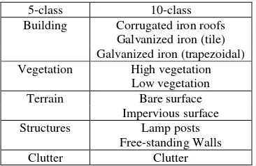
To develop the classification algorithm, ten 30 x 30 m2 tiles were selected in the study area in such a manner as to display the heterogeneity of the objects in the settlement. The first classification identifies the main objects in the area (Table 1). The second classification targets more specific semantic attributes which could be of interest for upgrading projects. For example, different types of roof material may be an indicator for construction quality, the presence of street lights are important for the sense of security in the area, and free-standing walls may indicate plot boundaries. The clutter class consists of temporary objects on the terrain, such as cars, motorbikes, clothes lines with drying laundry, and other miscellaneous objects. A training set of 1000 pixels distributed over all ten tiles was collected. Reference data was created by manually labelling pixels according to the 10-class problem. These labels were aggregated to the 5-class labels as indicated in Table 1. In cases where the orthomosaic clearly indicated terrain, but the type of terrain was unknown (e.g. due to shadowed footpaths between buildings), the points were included in the reference data of the 5-class but not the 10-class problem. In total, approximately 89.1% of the image tile pixels were labelled according to the 5 classes. The class of the remaining pixels was difficult to identify visually and so they were left unlabelled.
5-class 10-class
Building Corrugated iron roofs Galvanized iron (tile)
Table 1. Classes defined in the two classification problems.
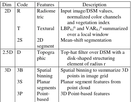
2.2 2D and 2.5D feature extraction from the orthomosaic and DSM
2D radiometric, textural, and segment-based features were extracted from the orthomosaic, and 2.5D topographical features were extracted from the DSM (see the overview in Table 2). The radiometric features consisted of the input R, G, and B colour channels as well as the normalized values r, g, and b, calculated by dividing the colour channel by the sum of all three channels. The excess green (ExG(2)) vegetation index (Woebbecke et al., 1995) was also calculated, as Torres-Sánchez et al. (2014) indicated that this vegetation index compared favourably to other indices for vegetation fraction mapping from UAV imagery. ExG(2) is calculated as follows:
Where r, g and b are the normalized RGB channels described above.
Applying a top-hat mathematical morphological filter to a DSM will give the height of a pixel above the lowest point within the area delimited by a structuring element. The size of the structuring element must be large enough to cover the entire object in question, but small enough to maintain the variation present in surface topography (Kilian et al., 1996). This size can be set in an automatic way based on granulometry to target a specific type of object such as buildings (Li et al., 2014). However, as the present classification problem targets objects of varying sizes, a circular top-hat filter is applied multiple times using structuring elements of varying radii r : from 0.25 to 1.0 m at 0.25 m intervals, and from 1 to 10 m at 1 m intervals. Previous research has shown such an approach applying DSM top-hat higher than the centre pixel and 0 if it is lower, defining a binary code of 2N bits. Rotational invariance is achieved by applying a circular shift, or bitwise rotation, to the code to obtain the minimal binary value. To reduce the number of unique codes, uniform patterns are defined as the codes containing a maximum of two binary 0/1 transitions. This allows for the definition of N+2 uniform, rotationally-invariant binary patterns, each of which can be assigned a unique integer. These LBP features are denoted as � �,���� . For a more detailed description of the calculation of LBP texture features see Ojala et al. (2002). Due to the binary nature of these patterns, they fail to capture the contrast between the centre pixel and its neighbours. Therefore, Ojala et al. (2002) recommend combining various � �,���� operators with a variance measure VARN,R (2), which compares the grayscale values of each neighbour (gN) to the average grayscale value in the local neighbourhood (µ).
� �,�=�∑�−�= ��− � , ℎ� � � =�∑�−�= �� (2)
To describe the local texture using LBPs, a sliding window is applied to the orthomosaic to locally compute the relative occurrence of each N+2 pattern. Here, we apply two sliding windows, one of 3x3 pixels and the other 10x10 pixels. For this analysis, the standard LBP combination described in Ojala et al. (2002) were utilized, consisting of: � 8,��� ., � ���6, ., � ���, ., and the corresponding VAR features.
The orthomosaic was segmented using the mean shift algorithm (Comaniciu and Meer, 2002). The algorithm transforms the RGB color values into L*u*v colorspace, and applies a kernel function to identify modes in the data. The algorithm requires two parameters to define the kernel bandwidths: hs which represents the spatial dimension, and hr which represents the spectral dimension (Comaniciu and Meer, 2002). These parameters were set to 20 and 5 respectively, based on experimental analysis. The segment features included in the classification consisted of the pixel-based radiometric features (i.e. R, G, B, r, g, b and ExG(2) ) averaged over each segment.
2.3 Feature extraction from the 3D point cloud
To include features from the point cloud in the classification, spatial binning was first applied to obtain: (i) the number of points per bin, (ii) the maximal height difference, and (iii) the standard deviation of the heights of all the points falling into the bin. The geographical grid used to define the bins was determined by the orthomosaic, so that each bin was exactly aligned to an image pixel. To reduce the number of empty bins, the attributes of each point were assigned to the corresponding bin and the 8 directly neighbouring pixels.
Planar segments in point clouds have demonstrated their usefulness in the identification of building roofs and walls in urban scenes (Vosselman, 2013). The planar segment features were obtained by applying a surface growing algorithm to the point cloud using a 1.0 m radius and a maximum residual of 30 cm. The segment number of the highest point per bin was used to assign the segment features to the pixel. This was based on the premise that if there are multiple layers in a point cloud (terrain and an overhanging roof, for example), it is the highest point in the point cloud (i.e. corresponding to the roof) which will be visible in the orthomosaic. For each segment, the number of points per segment, average residual, and inclination angle were calculated. Furthermore, the maximal height difference per bin of the segment (from the previous spatial binning features) was assigned to the entire segment. A nearest neighbour interpolation was utilized to assign a segment number, and the corresponding segment features, to empty pixels. Segment features were only calculated for segments which were identified at least once as being the highest segment in a bin, but all of the segment points pertaining to that segment were included in the calculation of the segment features.
The final step was to add more descriptive 3D-shape attributes from the point cloud into the image. Weinmann et al. (2015) present a set of 21 generic point cloud features. First, the optimal neighbourhood was calculated for each point by iteratively increasing the number of neighbouring points in a 3D k-nn search to maximize the Shannon entropy of the normalized eigenvalues (e1, e2, and e3) of the 3D covariance matrix (3).
��= −� ln � − � ln � − � ln � (3)
In this case, a minimum of 10 and maximum of 100 neighbours were selected, as suggested by Weinmann et al. (2015) and Demantké et al. (2011). Using this optimal neighbourhood size, Dim Code Features Description
Top-hat filter over DSM with a disk-shaped structuring
3D geometric, 3D shape, and 2D shape features were calculated. The 3D geometric features consisted of the maximum altitude difference and standard deviation of the height values of neighbouring points. The absolute maximum altitude feature was excluded, as the study area is sloped. From the 3D covariance matrix, combinations of the normalized eigenvectors are used to describe the linearity �� (4), planarity � (5), scattering � (6), omnivariance (7), anisotropy (8), eigenentropy (9), sum eigenvalues (10), and change of curvature (11).
��= � − � /� (4) binning features described by the framework were not applied, as they are similar to those calculated previously. To speed up computation speed, these 3D features were only calculated for the highest 3D point per pixel identified in the spatial binning step, again assuming that the highest point will represent the object which is visible in the UAV orthomosaic.
2.4 Feature selection and classification
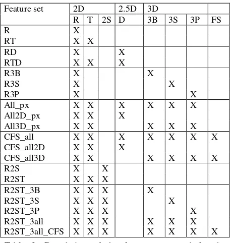
Feature sets are grouped based on the input data used to calculate the features (2D orthomosaic, 2.5D DSM, or 3D point cloud), the application of a feature selection algorithm, and whether or not image-based segment features are included (Table 3). The first two groups simulate practices which use either the orthomosaic and DSM or point cloud features and RGB information to classify the scene. The next two groups represent an integration of various point-cloud based features into the image grid. To reduce the
computational cost and prevent over-fitting the classifier, the Correlation-Based Feature Selector (CFS) is also applied to these sets. It is a multi-variate feature selector, screening features for a maximal correlation with the class while reducing redundancy between features. It was utilized with a best first forward feature selection, stopping when five consecutive iterations show no improvement regarding the correlation heuristic (Hall, 1999).
For all the previous sets, the features are summarized per pixel of the image grid. However, the sixth group of feature sets also includes the Mean Shift segment radiometric features. This includes a feature set (R2ST) where the mean-shift segments are used to summarize the LBP textures into normalized histograms, rather than the moving window. Finally, there are feature sets which integrate both pixel-based, segment-based, and point-cloud based features. In this case, image-based segments are again used to summarize the information from the 3D features.
The supervised classification is performed using a SVM classifier with an RBF kernel implemented in LibSVM (Chang and Lin, 2011). SVM classifiers maximize the margins between classes while minimizing training errors, a method which is proven to obtain high classification results and generalization capabilities even when few training samples are utilized (Bruzzone and Persello, 2010). To train the SVM classifiers, all the features were normalized to a 0-1 interval. Then, a 5-fold cross-validation was used to optimize the values of the soft margin cost function C from 2-5 to 215 and the spread of the Gaussian kernel γ from 2 -12 to 23 on the training set.
The classification results are compared using the Overall Accuracy (OA) of the prediction maps compared to the reference data. Furthermore, confusion matrices as well as the correctness (12) and completeness (13) are used to compare the relations between number of true positives (TP), false negatives (FN) and false positives (FP) per class.
� � =��+���� (12)
� � � =��+���� (13)
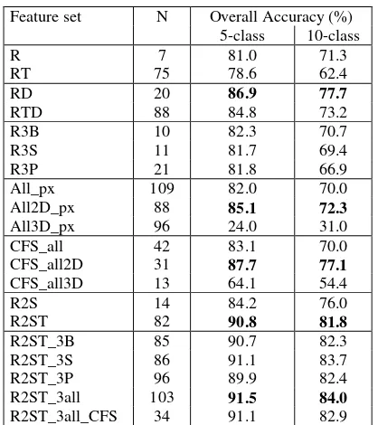
3. RESULTS
The classification overall accuracy using the various feature classes is presented in Table 4, with the completeness and correctness of the 5-class and 10-class problems displayed in Tables 5 and 6, and 7 and 8 respectively. We first compare the feature sets which utilize only pixel-based information, similar to the combination of pixel spectra with elevation maps common to methods making use of LiDAR and multi-spectral imagery. When using only the DSM and RGB image for a pixel-wise classification, the combination of radiometric information with the set of DSM top-hat features (RD) clearly obtains the best results (Table 4), with an OA of 77.7% for the 10-class problem and 86.9% for the 5-class problem. The inclusion of point-cloud features to each individual pixel does not achieve the same accuracy as the cases which utilize DSM information. Even when including all the 2D and 2.5D (All2D_px) and 3D (All_px) does not improve the classification results. This is likely due to the inclusion of features which are not relevant for the classification, as using the CFS feature selection method improves the classification accuracy. A CFS applied to the 2D radiometric and textural and 2.5D topographical features (CFS_all2D) achieves the highest accuracy (87.7%) in the 5-class problem for all pixel-based methods, though it is still achieves a lower accuracy than the RD feature set in the 10-class problem.
The integration of segment-based features in addition to the point-based features significantly improves the classification results. The 5-class OA jumps from 87.7% for CFS_all2D to 90.8% for R2ST which uses the mean-shift segments to compute the LBP-feature normalized histograms. The 10-class OA is also higher, 81.8% in this case compared to maximum of 77.7% when not including the mean-shift segment features. If the spatial binning, planar segment, and 3D geometric features from the point cloud are also summarized by the segments (R2ST_3all), we achieve the highest OA of 84.0% in the 10-class problem and 91.5% in the 5-class problem. The largest gain of including the planar segment 3D information (R2ST_3S) is observed in the 10-class problem by reducing the confusion between tile and corrugated iron roofs, low vs high vegetation, and bare surface
versus corrugated iron roofs, as well as improving the identification of walls (Tables 7 and 8). The point-based 3D shape features (R2ST_3P) improved the identification of lamp posts.
The results also illustrate which classes remain difficult to identify. In the 5-class classification problem, the structure and clutter classes are often confused with building and terrain. The correctness was 0.26 for structures and 0.27 for clutter using the R2ST_3all feature set (Table 5). The completeness of these classes was better, achieving values of 0.66 and 0.58 respectively when using the R2ST_3all feature set (Table 6). Structures were most often confused with building roofs and clutter was most often assigned to terrain pixels. Nonetheless, the correctness and completeness of the building, vegetation, and terrain classes was more than 0.88 for all features sets which included the mean-shift segment features. The R2ST_3all identified building pixels with a correctness of 0.98 and a completeness of 0.94.
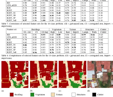
The 10-class problem displayed difficulties in identifying lamp posts, walls, type of terrain, and high- versus low-vegetation. Interestingly, the RD feature set obtained the highest completeness for the lamp post class. As lamp posts have a standard size, these objects were relatively easily recognized by the DSM top-hat features. The correctness was still only 0.14, due to the confusion between lamp posts and protruding tree branches of a similar planimetric dimension. The R2ST_3all feature set had the second highest completeness for lamp posts at 0.98, and the highest correctness at 0.31. Corrugated iron roofs were often misclassified as walls, most likely because the overlapping iron sheets sometimes displayed narrow white rectangular patches similar to free-standing walls in the scene (Figure 1). Walls were best identified by the R2ST_3S, R2ST_3P, and R2ST_3all feature sets, which is possibly due to the inclusion of planarity and normal inclination angle features in the planar segment and local shape features. Regarding the terrain classes, results indicate that for all feature sets, there was much confusion between bare terrain and impervious surfaces. This is a common problem in remote sensing, as shadows from surrounding buildings and spectral similarity with pervious surfaces hinders the identification of impervious surfaces (Weng, 2012).
4. DISCUSSION
4.1 Importance of summarizing texture and 3D features over mean-shift segments
Out of all the feature sets, those which used a mean-shift segmentation to summarize texture or 3D features greatly increased the classification accuracy. The inclusion of local histogram texture features summarized by a moving window decreases the classification accuracy compared to only using radiometric features (i.e. RT vs. R in Table 4), but increases the accuracy when summarized according segment boundaries (i.e. R2ST vs. R2S in Table 4). As the extent of the moving window is fixed, it will summarize the textures of distinct classes at object borders, whereas this problem is avoided when using segments to summarize textural information. The discriminative power of the LBP texture features summarized per segment is possibly due to the high resolution of the UAV imagery, in which the texture of the corrugated iron roofs is clearly visible. This facilitates the distinction between building roofs, wall structures, and terrain. It is especially notable if one takes into account that for the R2ST feature set, no features derived from the DSM or point cloud are included, and yet it achieves a high classification accuracy.
decrease noise in the point cloud, such as outliers formed by dense matching errors. The R2ST_3all feature set proves the utility of integrating both 2D and 3D features, especially in the context of the 10-class problem.
4.2 Propagation of errors when using DSM features Regarding the pixel-based methods, the suite of DSM top-hat filters allows for the distinction of objects of various sizes, which could be used to target elevated objects of uniform size. However, errors in the DSM are then propagated to the classification. For example, in this case the Pix4D software utilized an Inverse Distance Weighting (IDW) interpolation incorporated to create the DSM, which causes the terrain next to or footpaths between buildings to be misclassified as building or vegetation since these pixels are falsely assigned a higher elevation value. This hinders the suitability of the classification for upgrading projects, which requires the delineation of individual buildings or identification of footpaths to analyse accessibility in the settlement. As the building outlines are clearly visible in the orthophoto, the mean-shift segmentation improves the delineation of building outlines, especially when combined with 3D features. Therefore, the use of 3D features summarized
per image segment has a better classification performance than the features extracted from the DSM.
4.3 Comparison of the three sets of 3D features
Three groups of features were derived from the point cloud to represent 3D attributes: spatial binning, planar segment features, and 3D point features. Spatial binning is the easiest method to implement and improves the identification of lamp posts (R2ST_3B) as opposed to not using 3D features (R2ST). However, the inclusion of more sophisticated 3D features such as planar segment or point-based 3D shape features obtain better results. The inclusion of planar segments had the single largest benefit (compared with spatial binning or point-based shape features), as indicated by Table 4. In informal settlements, a single roof may consist of patches of materials displaying heterogeneous characteristics causing an over-segmentation of the mean shift based on radiometric features. However, these different materials may still generally lie on the same plane, allowing the 3D planar segments to summarize information over a larger area of the roof. However, errors in the point cloud segmentation, such as building roofs and terrain being assigned to the same plane in sloped areas, caused visible artefacts in the
Feature set Buildings Vegetation Terrain Structures Clutter
GI – tile CI GI-trap High Low Bare Imperv. Lamps Walls Clutter
RD 0.90 0.92 0.91 0.88 0.37 0.75 0.74 0.14 0.14 0.13
CFS_all2D 0.78 0.95 0.97 0.86 0.32 0.78 0.77 0.03 0.12 0.13
R2S 0.74 0.95 0.99 0.91 0.34 0.75 0.70 0.11 0.08 0.13
R2ST 0.84 0.96 0.99 0.93 0.43 0.79 0.83 0.10 0.21 0.14
R2ST_3S 0.89 0.97 0.99 0.94 0.48 0.83 0.80 0.11 0.27 0.18
R2ST_3B 0.89 0.96 1.00 0.95 0.44 0.79 0.84 0.19 0.19 0.16
R2ST_3P 0.91 0.96 0.98 0.93 0.44 0.79 0.84 0.30 0.22 0.17
R2ST_3all 0.97 0.96 1.00 0.90 0.45 0.78 0.85 0.31 0.30 0.18
Table 7. Correctness of selected feature sets for the 10-class problem. (GI = galvanized iron, CI = corrugated iron, Imperv. = impervious)
Feature set Buildings Vegetation Terrain Structures Clutter
GI – tile CI GI-trap High Low Bare Imperv. Lamps Walls Clutter
RD 0.82 0.91 0.95 0.65 0.89 0.58 0.62 0.99 0.64 0.43
CFS_all2D 0.74 0.88 0.85 0.64 0.59 0.64 0.65 0.57 0.53 0.67
R2S 0.78 0.83 0.91 0.66 0.72 0.71 0.62 0.57 0.45 0.62
R2ST 0.82 0.91 0.93 0.70 0.75 0.78 0.66 0.62 0.55 0.61
R2ST_3S 0.86 0.93 0.93 0.73 0.79 0.77 0.68 0.64 0.62 0.72
R2ST_3B 0.81 0.91 0.93 0.69 0.78 0.76 0.70 0.70 0.57 0.66
R2ST_3P 0.80 0.92 0.93 0.76 0.73 0.73 0.67 0.76 0.64 0.75
R2ST_3all 0.85 0.94 0.92 0.76 0.82 0.69 0.67 0.98 0.63 0.77
Table 8. Completeness of selected feature sets for the 10-class problem. (GI = galvanized iron, CI = corrugated iron, Imperv. = impervious)
(a) (b) (c) (d)
Building Vegetation Terrain Structures Clutter
classification. The 3D point attributes had the highest impact on the correct classification of lamp posts, greatly reducing confusion with corrugated iron roofs. The integration of all 3D features (R2ST_all) has the highest performance, suggesting that the different 3D features provide complimentary information. Furthermore, although the feature selection algorithm increased the performance of the pixel-based classification, it did not enhance performance for the features set containing the combination of all radiometric, mean-shift segment, and 3D features.
4.4 Remaining difficulties
Although the classification obtained a high overall accuracy of 91.5% on the 5 class problem and 84% on the 10 class problem, there were a number of classes which remain difficult to distinguish. All feature sets displayed a high confusion between low- vs. high-vegetation and bare vs. impervious surfaces. The former could be due to the characteristics of the scene, where grasses on steep slopes may mimic some of the characteristics of high vegetation: e.g. green, rounded shape, large height differences. Bare vs. impervious surfaces were also difficult to distinguish as many impervious surfaces may be partially covered in dirt and due to shadows. Furthermore, red-painted roofs and rusted iron sheets tend to be spectrally similar to the bare soils which tend to be reddish in colour. Other inaccuracies may be due to the definition reference data using the orthomosaic. Some objects, such as overhanging electricity wires, are not visible in the orthomosaic. This causes a misalignment in the 3D features computed in the point cloud and the 2D-derived reference data. Finally, it is also important to note that the current classification uses approximately 0.01% of the reference pixels for training the SVM model. Increasing the training set size could also improve classification accuracy.
5. CONCLUSIONS AND RECOMMENDATIONS This work illustrates the importance of integrating 2D radiometric, textural, and segment features, 2.5D topographical features, and 3D geometrical features for informal settlement classification. Through the integration of these features, a high classification accuracy can be obtained, despite the challenging characteristics of the study area, which consists of small buildings, mixed and poor quality roof materials with clutter located on steep slopes. Various feature sets were applied to a 5-class problem: buildings, vegetation, terrain, structures (free-standing walls and lamp posts), and clutter (cars, laundry lines, miscellaneous objects on the ground); and a 10-class problem which distinguished roof material, high/low vegetation, pervious/impervious surfaces, and type of structure. Results indicate that using 2D radiometric features together with a series of top-hat morphological filters applied to the DSM had the highest accuracy of all pixel-based feature sets. However, inaccuracies in the DSM are propagated into the classification. Summarizing texture features over mean-shift segments obtains an improved classification even though it only requires the 2D RGB image as input. However, the best results are obtained when integrating point-based and segment-based 3D features from the point cloud with image-based radiometric and texture features summarized over segments. Especially in the more complex 10-class problem, the necessity of more sophisticated feature sets including 3D features is evident (raising the OA from 81.8% to 84.0%). 3D planar segment features facilitated the identification of walls and clutter, while point-based 3D shape attributes facilitated the classification of lamp posts.
The observation that the highest classification accuracies were obtained by combining both 2D and 3D features demonstrates that both feature spaces contain complimentary information. As UAV imagery provides both a dense 3D point cloud and a high-resolution orthomosaic, both can be exploited to improve scene understanding. This is especially important in challenging scenes such as informal settlements, where many assumptions fundamental to building extraction algorithms (such as ground planarity and free-standing buildings) do not hold. Here, we demonstrate which feature sets can be combined to provide an accurate, up-to-date classification map of informal settlements, which is essential for upgrading projects. It also demonstrates the importance of using 3D features directly, which preserves narrow footpaths between buildings which may be lost if using features from interpolated DSMs. This is crucial in the context of informal settlement upgrading, as the narrow footpaths provide important information regarding the accessibility of houses to utilities and services. Other studies can use the current findings to direct their attention to certain feature sets according to the target classes of their specific classification problem.
Further research focus on an analysis of how to fine-tune these features to enhance the recognition of various objects and materials in informal settlements. The synergies between 3D features obtained through spatial binning, planar segments and 3D shape features could also be further investigated, analysing in which specific cases one or the other should be applied also considering the computational efforts. Application of this framework to different study areas could provide insights regarding the transferability and sensitivity to parameter tuning of the different features. Classification post-processing, which was considered outside the scope of the present study, could also reduce the presence of small pixel groups and improve the classification results.
REFERENCES
Arefi, H., Hahn, M., 2005. A hierarchical procedure for segmentation and classification of airborne LIDAR images. In: International Geoscience and Remote Sensing Symposium, Vol 7. pp. 49-50.
Barry, M., Rüther, H., 2005. Data collection techniques for informal settlement upgrades in Cape Town, South Africa. URISA Journal. 17(1), pp. 43-52.
Bruzzone, L., Persello, C., 2010. Approaches Based on Support Vector Machines to Classification of Remote Sensing Data. In: Chen, C.H. (Eds.), Handbook of Pattern Recognition and Computer Vision, fourth ed. World Scientific, Singapore, pp. 329-352.
Chang, C.-C., Lin, C.-J., 2011. LIBSVM: A library for support vector machines. ACM Transactions on Intelligent Systems and Technology. 2(3), pp. 27:21-27:27.
Comaniciu, D., Meer, P., 2002. Mean shift: A robust approach toward feature space analysis. Pattern Analysis and Machine Intelligence, IEEE Transactions on. 24(5), pp. 603-619.
Demantké, J., Mallet, C., David, N., Vallet, B., 2011. Dimensionality based scale selection in 3D lidar point clouds. International Archives of Photogrammetry, Remote Sensing and Spatial Information Sciences, Laser Scanning. Vol. XXXVIII-5/W12, pp. 97-102.
classification using Random Forests. ISPRS Journal of Photogrammetry and Remote Sensing. 66(1), pp. 56-66.
Hall, M.A., 1999. Correlation-based feature selection for machine learning. The University of Waikato.
Hartfield, K.A., Landau, K.I., Van Leeuwen, W.J., 2011. Fusion of high resolution aerial multispectral and LiDAR data: Land cover in the context of urban mosquito habitat. Remote Sensing. 3(11), pp. 2364-2383.
Huang, M.-J., Shyue, S.-W., Lee, L.-H., Kao, C.-C., 2008. A knowledge-based approach to urban feature classification using aerial imagery with lidar data. Photogrammetric Engineering & Remote Sensing. 74(12), pp. 1473-1485.
Kilian, J., Haala, N., Englich, M., 1996. Capture and evaluation of airborne laser scanner data. International Archives of Photogrammetry and Remote Sensing. Vol. XXXI, Part B3, pp. 383-388.
Kuffer, M., Barros, J., Sliuzas, R.V., 2014. The development of a morphological unplanned settlement index using very-high-resolution (VHR) imagery. Computers, Environment and Urban Systems. 48. pp. 138-152.
Li, Y., Zhu, L., Tachibana, K., Shimamura, H., 2014. Morphological Operation Based Dense Houses Extraction From DSM. International Archives of the Photogrammetry, Remote Sensing and Spatial Information Sciences. Vol. XL-3, pp. 183-189.
Longbotham, N., Chaapel, C., Bleiler, L., Padwick, C., Emery, W.J., Pacifici, F., 2012. Very high resolution multiangle urban classification analysis. Geoscience and Remote Sensing, IEEE Transactions on. 50(4), pp. 1155-1170.
Myint, S.W., Gober, P., Brazel, A., Grossman-Clarke, S., Weng, Q., 2011. Per-pixel vs. object-based classification of urban land cover extraction using high spatial resolution imagery. Remote Sensing of Environment. 115(5), pp. 1145-1161.
Ojala, T., Pietikainen, M., Maenpaa, T., 2002. Multiresolution gray-scale and rotation invariant texture classification with local binary patterns. Pattern Analysis and Machine Intelligence, IEEE Transactions on. 24(7), pp. 971-987.
Priestnall, G., Jaafar, J., Duncan, A., 2000. Extracting urban features from LiDAR digital surface models. Computers, Environment and Urban Systems. 24(2), pp. 65-78.
Pugalis, L., Giddings, B., Anyigor, K., 2014. Reappraising the World Bank responses to rapid urbanisation: Slum improvements in Nigeria. Local Economy. 29(4-5), pp. 519-540.
Rottensteiner, F., Sohn, G., Gerke, M., Wegner, J.D., Breitkopf, U., Jung, J., 2014. Results of the ISPRS benchmark on urban object detection and 3D building reconstruction. ISPRS Journal of Photogrammetry and Remote Sensing. 93, pp. 256-271.
Serna, A., Marcotegui, B., 2014. Detection, segmentation and classification of 3D urban objects using mathematical morphology and supervised learning. ISPRS Journal of Photogrammetry and Remote Sensing. 93, pp. 243-255.
Taubenböck, H., Kraff, N.J., 2013. The physical face of slums: a structural comparison of slums in Mumbai, India, based on remotely sensed data. Journal of Housing and the Built Environment. 29(1), pp. 15-38.
Torres-Sánchez, J., Peña, J., De Castro, A., López-Granados, F., 2014. Multi-temporal mapping of the vegetation fraction in early-season wheat fields using images from UAV. Computers and Electronics in Agriculture. 103, pp. 104-113.
UN-Habitat, 2012. Streets as tools for urban transformation in slums: A Street-led Approach to Citywide Slum Upgrading, Nairobi, p. 85.
Vosselman, G., 2013. Point cloud segmentation for urban scene classification. ISPRS-International Archives of the Photogrammetry, Remote Sensing and Spatial Information Sciences. 1(2), pp. 257-262.
Weidner, U., Förstner, W., 1995. Towards automatic building extraction from high-resolution digital elevation models. ISPRS Journal of Photogrammetry and Remote Sensing. 50(4), pp. 38-49.
Weinmann, M., Jutzi, B., Hinz, S., Mallet, C., 2015. Semantic point cloud interpretation based on optimal neighborhoods, relevant features and efficient classifiers. ISPRS Journal of Photogrammetry and Remote Sensing. 105, pp. 286-304.
Weng, Q., 2012. Remote sensing of impervious surfaces in urban areas: Requirements, methods, and trends. Remote Sensing of Environment. 117, pp. 34-49.
Woebbecke, D., Meyer, G., Von Bargen, K., Mortensen, D., 1995. Color indices for weed identification under various soil, residue, and lighting conditions. Transactions of the ASAE. 38(1), pp. 259-269.
Xu, S., Vosselman, G., Oude Elberink, S., 2014. Multiple-entity based classification of airborne laser scanning data in urban areas. ISPRS Journal of Photogrammetry and Remote Sensing. 88, pp. 1-15.