EVALUATING THE VARIATIONS IN THE FLOOD SUSCEPTIBILITY MAPS
ACCURACIES DUE TO THE ALTERATIONS IN THE TYPE AND EXTENT OF THE
FLOOD INVENTORY
M. SH. Tehrany a, *, S. Jones aa
Geospatial Science, RMIT University, Melbourne, VIC, 3000, Australia - (mahyat.shafapourtehrany, simon.jones)@rmit.edu.au
KEY WORDS: Flood, Hazard Mapping, Inventory Map, Logistic Regression, Australia
ABSTRACT:
This paper explores the influence of the extent and density of the inventory data on the final outcomes. This study aimed to examine the impact of different formats and extents of the flood inventory data on the final susceptibility map. An extreme 2011 Brisbane flood event was used as the case study. LR model was applied using polygon and point formats of the inventory data. Random points of 1000, 700, 500, 300, 100 and 50 were selected and susceptibility mapping was undertaken using each group of random points. To perform the modelling Logistic Regression (LR) method was selected as it is a very well-known algorithm in natural hazard modelling due to its easily understandable, rapid processing time and accurate measurement approach. The resultant maps were assessed visually and statistically using Area under Curve (AUC) method. The prediction rates measured for susceptibility maps produced by polygon, 1000, 700, 500, 300, 100 and 50 random points were 63%, 76%, 88%, 80%, 74%, 71% and 65% respectively.
Evidently, using the polygon format of the inventory data didn’t lead to the reasonable outcomes. In the case of random points, raising the number of points consequently increased the prediction rates, except for 1000 points. Hence, the minimum and maximum thresholds for the extent of the inventory must be set prior to the analysis. It is concluded that the extent and format of the inventory data are also two of the influential components in the precision of the modelling.
* Corresponding author
1. INTRODUCTION
The combined influence of human activities and climate change are the main factors that trigger catastrophic flood (Sakamoto et al., 2007; Zhang et al., 2014). Although it is not possible to avoid natural hazard occurrences completely, most susceptible regions can be recognized and controlled in order to mitigate the negative impacts of the future events (Vis et al., 2003). Flood management can be categorized into several stages: susceptibility, hazard, vulnerability and risk analysis (Sharma et al., 2010). The primary need in performing any sort of flood modelling is having a flood inventory map and a set of flood causative factors (Tehrany et al., 2013). The necessity of producing flood inventory maps is to record and document the size, coverage and trend of the inundated areas. Inventory maps can be used for different purposes (Guzzetti et al., 2012), including: documentation and record keeping (Trigila et al., 2010), damage and cost assessments (Brenner et al., 2016), as an initial stage in further flood assessments (Pradhan et al., 2017) etc. Historical flood events can be mapped using traditional and advanced techniques (Giustarini et al., 2013). Traditional approaches require the considerable time and resources (Auynirundronkool et al., 2012). On the other hand, advances in GIS and Remote Sensing (RS) technologies which brought new insight into natural hazard domain resolved those difficulties (Jones and Reinke, 2009). Visual interpretation of the aerial photographs (Schumann et al., 2011), segmentation and texture analysis of Radar imageries (Pradhan et al., 2014), change detection approaches (Pradhan et al., 2016) etc. are some examples of advanced techniques in detecting and mapping the flooded regions.
Despite flood hazard maps being compiled using different types of algorithms and techniques, limited attempts have been made to compare the flood susceptibility maps produced using different inventory types and extents. In most studies the user-defined values are utilized as inventory locations for the modelling purpose (Galli et al., 2008). Reason is that there is no agreement existed that defines the sufficient extent of the inventory locations or the format of it in order to have a reliable final prone areas map. This research aims to examine the impact of various extents of the flood inventory on the accuracy of the final susceptibility maps. In addition, the inventory data was used in two formats of polygon and point to evaluate their impact on the final outcomes.
LR is one of the most popular statistical methods in natural hazard mapping, such as flood (Pradhan, 2010), forest fire (Pourghasemi, 2016), landslide (Umar et al., 2014), land subsidence (Hu et al., 2009) etc. LR is a Multivariate Statistical Analysis (MSA) algorithm which extracts the regression correlation among a binary dependent variable (i.e. flood inventory) and several independent variables (i.e. flood causative factors) (Tehrany et al., 2015). Subsequently, it predicts the existence and non-existence of an event (future flooding) based on those correlations. All sorts of data such as nominal, categorized, scale or a combination of them are acceptable by LR. Moreover, this method does not require any assumptions to be defined prior to the analysis (Umar et al., 2014). The flood probability index can be calculated using the equation 1:
z e
p
1 1
(1)
where p= probability of the event z= linear combination
z is the linear combination and it follows that logistic regression involves fitting an equation of the following form to the data:
n nx b x b x b x b b
z 0 11 2 2 3 3 (2) where p = intercept of the method (constant value)
) ,..., 2 , 1 , 0
(n n
bn = LR measured coefficients )
,..., 2 , 1 , 0
(n n
xn = flood causative factors
2. STUDY AREA AND DATA USED
Several extreme precipitation events occurred in Australia between 2010 and 2011 which caused destructive floods. Seventy-eight percent of the State of Queensland was affected by the flood event that took place in January 2011 (Inquiry and Holmes, 2012). An estimated 200,000 people were affected throughout Queensland during this period causing an estimated
$5 Billion worth of damage
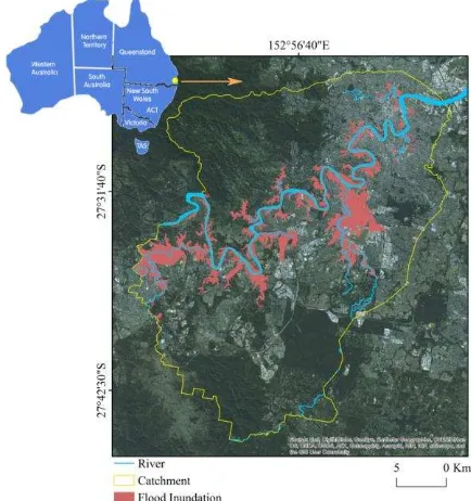
(http://www.bom.gov.au/qld/flood/fld_history/brisbane_history. shtml). Brisbane was one of the most affected citied in Queensland receiving over $500 millions of damage (Chanson et al., 2014; van den Honert and McAneney, 2011) due to this event (Figure 1). This study focuses on the Brisbane River Catchment in Queensland, Australia. It is located between 152°46'6.974"E 27°24'33.175"S and 153°5'55.797"E 27°45'30.227"S, and is some 760 km2 in area. The catchment is the mixture of urban, rural-forestry and grazing land.
Figure 1. Selected Brisbane river catchment, and the flooded regions
To build a flood susceptibility model two datasets of flood inventory and causative factors are required (Mojaddadi et al., 2017). Seven sets of flood inventory maps were prepared and used in the current flood susceptibility mapping. The first
inventory map was constructed using polygons representing the inundation regions (https://data.qld.gov.au/dataset). The other six inventory datasets were created using random points of 1000, 700, 500, 300, 100 and 50 derived from the polygons.
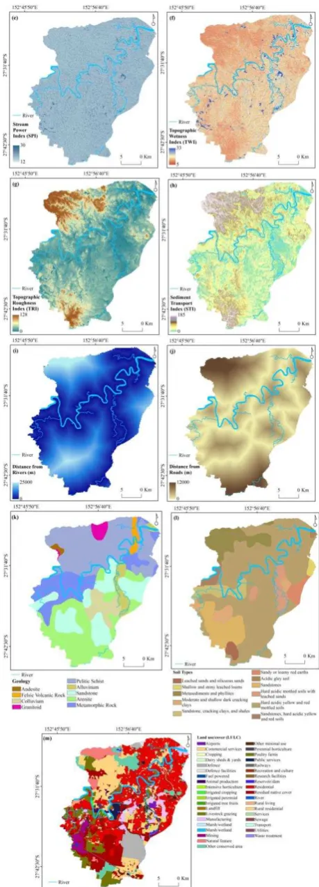
The flood causative factors dataset, altitude, slope, aspect, curvature, Stream Power Index (SPI), Topographic Wetness Index (TWI), Topographic Roughness Index (TRI), Sediment Transport Index (STI), distance from rivers, distance from road, geology, soil and land use/cover (LULC) were prepared and used from a variety of sources (Figure 2): A DEM with 5-meter spatial resolution was produced from Light Detection and Ranging (LiDAR) data provided by Australian Government (http://www.ga.gov.au/elvis/). This data was used to create topographical factors of slope, aspect, curvature, and hydrological factors of SPI, TWI, TRI and STI. Soil (1:250,000 scale) and geology (1:100,000 scale) were obtained from the CSIRO and Australian government websites. Clay and sandstone are the dominant soil types in the study area. A detailed LULC map was produced by the Queensland Land Use Mapping Program (QLUMP) and was provided by the Queensland Government. This LULC thematic map was created by classifying SPOT5 imagery, high spatial resolution orthophotography and scanned aerial photos and using local expert knowledge. All causative factors were formatted into raster with a 5 × 5 m pixel size. The Logistic Regression (LR) technique which was used for the modeling supports all kinds of data types; therefore, no classification analysis was required for the causative factors.
Figure 2. Flood causative factors(a) altitude, (b) slope, (c) aspect, (d) curvature, (e) SPI, (f) TWI, (g) TRI, (h) STI, (i) distance from river, (j) distance from roads, (k) geology, (l) soil
and (m) LULC
3. METHODOLOGY
All the flood causative factors and seven flood inventory maps were transformed from raster to ASCII format and transferred to SPSS Software to perform LR analyses. LR method was performed seven times and subsequently seven z equations (equation 2) were created. Finally, using equation 1 seven flood probability indexes were calculated. The stepwise methodology flowchart is shown in Figure 3.
Figure 3. Flowchart
4. RESULTS
LR coefficients were measured by evaluating the associations between seven inventory maps and thirteen flood causative factors. To acquire the flood probability maps, the calculated regression coefficient for each causative factor was entered in Eq. (2), yielding;
Inventory data used: polygons
084 . 1 log
) * 000001 . 0 ( ) * 05 9724 . 1 (
) * 061435635 .
0 ( ) * 015 . 0 (
) * 02388181 .
0 ( ) * 39492 021 . 0 (
) *
0003 . 0 ( ) * 000065 . 0 (
) * 14079016 .
0 ( ) * 001544911 .
0 (
LULC Soil y Geo
Road River
E
STI TRI
TW I SPI
Curvature Aspect
Slope Altitude
z
Inventory data used: 1000 random points
Inventory data used: 700 random points
31169
Inventory data used: 500 random points
9
Inventory data used: 300 random points
5
Inventory data used: 100 random points
6
Inventory data used: 50 random points
6
The measured z values were subsequently used in equation 1 in order to derive the final flood probability indexes. The
probabilities were then classified into five categories of “Very High”, “High”, “Moderate”, “Low” and “Very Low”
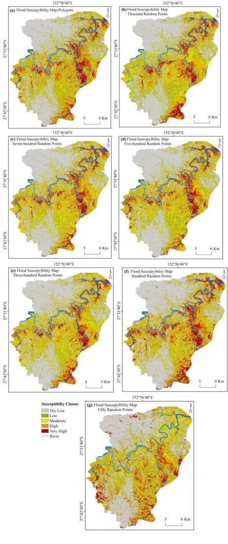
susceptibility zones to produce the flood susceptibility maps (Figure 4).
Figure 4. Flood susceptibility maps derived using seven inventories of: (a) polygons, (b) 1000 random points, (c) 700 random points, (d) 500 random points, (e) 300 random points,
(f) 100 random points and (g) 50 random points
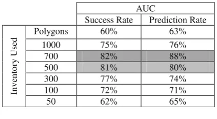
For the purpose of validation, area under curve (AUC) was used and both success and prediction rates were measured. AUC is a The International Archives of the Photogrammetry, Remote Sensing and Spatial Information Sciences, Volume XLII-4/W5, 2017
very popular way of comparing overall classifier performance and one of the most cited techniques in natural hazard researches (Jebur et al., 2015; Woods et al., 1997; Xu et al., 2014). The success and prediction accuracies of seven flood models were assessed qualitatively and presented in Table 1.
AUC
Success Rate Prediction Rate
In
v
en
to
ry
Us
ed
Polygons 60% 63%
1000 75% 76%
700 82% 88%
500 81% 80%
300 77% 74%
100 72% 71%
50 62% 65%
Table 1. AUC outcomes
The flood susceptibility maps derived from polygon, 1000, 700, 500, 300, 100 and 50 produced the success rates of 60%, 75%, 82%, 81%, 77%, 72% and 62% respectively, and the prediction rates of 63%, 76%, 88%, 80%, 74%, 71% and 65% respectively.
5. DISCUSSION
Visually, the least accurate map was produced by 50 random inventory points (Figure 4g), as most of the regions around the river have been classified as moderate, low and very low; while, in the reality those areas were the most affected places by 2011 flooding. In addition, this figure has the least similarity to the rest of the susceptibility maps derived in this study. Figure 4b which was produced using thousand random points illustrates apparent miss-classifications. Some regions have been detected as very high susceptible and other regions such as southwest of the catchment has been mapped as non-prone zone. Figure 4c, d and e represent almost similar classes of susceptibility. The very high flood susceptible regions presented in those maps are located around the river and at the South part of the study area.
Using the polygon format of the inventory clearly exaggerated the outcomes. It might be due to entering a huge amount of training data into the model which impacted on the performance of the algorithm. This also can be seen visually in the Figure 4. In the case of random points, using the minimum numbers of 50, 100 and 300, and maximum number of 1000 produced the least accurate results. We believe that both the polygon format and 1000 random points had the similar impact on the LR performance, and increasing the extent of the training data will not necessarily increase the precision of the outcomes. On the other hand limited number of inventory point (i.e. 50, 100 and 300) did not provide enough information for LR method to process the correlations among the inventory points and flood causative factors.
The range of 500-700 was found as an optimal range for the
random point’s density in this particular study. As a conclusion,
in the case of having a set of consistent flood causative factors and using the same modelling approach, the variation in the density and type of the inventory data can considerably influence the findings. It is suggested to consider this stage prior to any modelling and define the safe and accurate threshold for the inventory.
6. CONCLUSION
The type and extent of the inventory data received less attention compared to the method and the causative factors used in the literature. This research evaluated the impact of using different types and extents of the inventory data on the precision of the final flood susceptibility map. In this regard, the major 2011 flood event in Brisbane, Australia was used as the case study. Seven sets of inventory data was prepared, utilized and compared, including: polygons of the flooded areas, 1000, 700, 500, 300, 100 and 50 random points. Using LR statistical approach the correlation among the inventories and thirteen flood causative factors were recognized and seven flood susceptibilities with different accuracies were produced. The lowest prediction and success rates were acquired in the case of using the inventory as a polygon format and random points of 50, 100, 300 and 1000. On the other hand, the highest success rate of 82% and prediction rate of 88% were produced by 700 random inventory points. These findings can be used as a proof of this statement that by altering the type and density of the inventory data, the accuracy will be changed as well. It is wise to find the most accurate range of random points instead of running the model using user-defined values. Our aim for future study is to apply and examine the impact of multiple iterations at specific number of points on the precision of the final susceptibility map. For instance, in order to select 500 inventory point different sets of random points can be used and their outcomes can be compared.
REFERENCES
Auynirundronkool, K., Chen, N., Peng, C., Yang, C., Gong, J., Silapathong, C., 2012. Flood detection and mapping of the Thailand Central plain using RADARSAT and MODIS under a sensor web environment. Int. J. Appl. Earth Obs. Geoinf. 14, 245-255.
Brenner, C., Meisch, C., Apperl, B., Schulz, K., 2016. Towards periodic and time-referenced flood risk assessment using airborne remote sensing. J. Hydrol. Hydromech. 64, 438-447.
Chanson, H., Brown, R., McIntosh, D., 2014. Human body stability in floodwaters: the 2011 flood in Brisbane CBD, Proceedings of the 5th international symposium on hydraulic structures: engineering challenges and extremes. The University of Queensland.
Galli, M., Ardizzone, F., Cardinali, M., Guzzetti, F., Reichenbach, P., 2008. Comparing landslide inventory maps. Geomorphology 94, 268-289.
Giustarini, L., Hostache, R., Matgen, P., Schumann, G.J.-P., Bates, P.D., Mason, D.C., 2013. A change detection approach to flood mapping in urban areas using TerraSAR-X. IEEE Trans. Geosci. Remote Sens. 51, 2417-2430.
Guzzetti, F., Mondini, A.C., Cardinali, M., Fiorucci, F., Santangelo, M., Chang, K.-T., 2012. Landslide inventory maps: New tools for an old problem. Earth-Sci. Rev. 112, 42-66.
Hu, B., Zhou, J., Wang, J., Chen, Z., Wang, D., Xu, S., 2009. Risk assessment of land subsidence at Tianjin coastal area in China. Environ. Earth. Sci. 59, 269.
Inquiry, Q.F.C., Holmes, C., 2012. Queensland Floods Commission of Inquiry: Final Report. Queensland Floods Commission of Inquiry.
Jebur, M.N., Pradhan, B., Tehrany, M.S., 2015. Manifestation of LiDAR-derived parameters in the spatial prediction of landslides using novel ensemble evidential belief functions and support vector machine models in GIS. IEEE J. Sel. Top. Appl. Earth Obs. Remote Sens. 8, 674-690.
Jones, S., Reinke, K., 2009. Innovations in remote sensing and photogrammetry. Springer.
Mojaddadi, H., Pradhan, B., Nampak, H., Ahmad, N., Ghazali, A.H.b., 2017. Ensemble machine-learning-based geospatial approach for flood risk assessment using multi-sensor remote-sensing data and GIS. Geomat. Nat. Haz. Risk., 1-23.
Pourghasemi, H.R., 2016. GIS-based forest fire susceptibility mapping in Iran: a comparison between evidential belief function and binary logistic regression models. Scand. J. For. Res. 31, 80-98.
Pradhan, B., 2010. Flood susceptible mapping and risk area delineation using logistic regression, GIS and remote sensing. JOSH 9.
Pradhan, B., Hagemann, U., Tehrany, M.S., Prechtel, N., 2014. An easy to use ArcMap based texture analysis program for extraction of flooded areas from TerraSAR-X satellite image. Comput. Geosci. 63, 34-43.
Pradhan, B., Sameen, M.I., Kalantar, B., 2017. Optimized Rule-Based Flood Mapping Technique Using Multitemporal RADARSAT-2 Images in the Tropical Region. IEEE J. Sel. Top. Appl. Earth Obs. Remote Sens.
Pradhan, B., Tehrany, M.S., Jebur, M.N., 2016. A New Semiautomated Detection Mapping of Flood Extent From TerraSAR-X Satellite Image Using Rule-Based Classification and Taguchi Optimization Techniques. IEEE Trans. Geosci. Remote Sens. 54, 4331-4342.
Sakamoto, T., Van Nguyen, N., Kotera, A., Ohno, H., Ishitsuka, N., Yokozawa, M., 2007. Detecting temporal changes in the extent of annual flooding within the Cambodia and the Vietnamese Mekong Delta from MODIS time-series imagery. Remote Sens. Environ. 109, 295-313.
Schumann, G.J.-P., Neal, J.C., Mason, D.C., Bates, P.D., 2011. The accuracy of sequential aerial photography and SAR data for observing urban flood dynamics, a case study of the UK summer 2007 floods. Remote Sens. Environ. 115, 2536-2546.
Sharma, N., Johnson, F.A., Hutton, C.W., Clark, M.J., 2010. Hazard, vulnerability and risk on the Brahmaputra basin: a case study of river bank erosion. Open Journal of Hydrology 4, 211-226.
Tehrany, M.S., Pradhan, B., Jebur, M.N., 2013. Spatial prediction of flood susceptible areas using rule based decision tree (DT) and a novel ensemble bivariate and multivariate statistical models in GIS. J. Hydrol. 504, 69-79.
Tehrany, M.S., Pradhan, B., Jebur, M.N., 2015. Flood susceptibility analysis and its verification using a novel
ensemble support vector machine and frequency ratio method. Stoch. Environ. Res. Risk. Assess. 29, 1149-1165.
Trigila, A., Iadanza, C., Spizzichino, D., 2010. Quality assessment of the Italian Landslide Inventory using GIS processing. Landslides 7, 455-470.
Umar, Z., Pradhan, B., Ahmad, A., Jebur, M.N., Tehrany, M.S., 2014. Earthquake induced landslide susceptibility mapping using an integrated ensemble frequency ratio and logistic regression models in West Sumatera Province, Indonesia. Catena 118, 124-135.
van den Honert, R.C., McAneney, J., 2011. The 2011 Brisbane floods: causes, impacts and implications. Water 3, 1149-1173.
Vis, M., Klijn, F., De Bruijn, K., Van Buuren, M., 2003. Resilience strategies for flood risk management in the Netherlands. Intl. J. River. Basin. Management. 1, 33-40.
Woods, K., Kegelmeyer, W.P., Bowyer, K., 1997. Combination of multiple classifiers using local accuracy estimates. IEEE Trans. Pattern Anal. Mach. Intell. 19, 405-410.
Xu, L., Li, J., Brenning, A., 2014. A comparative study of different classification techniques for marine oil spill identification using RADARSAT-1 imagery. Remote. Sens. Environ. 141, 14-23.
Zhang, Q., Gu, X., Singh, V.P., Xiao, M., 2014. Flood frequency analysis with consideration of hydrological alterations: Changing properties, causes and implications. J. hydrol. 519, 803-813.