A COMPARISON OF SIMULATED ANNEALING, GENETIC ALGORITHM AND
PARTICLE SWARM OPTIMIZATION IN OPTIMAL FIRST-ORDER DESIGN OF
INDOOR TLS NETWORKS
F. Jia a, *, D. Lichti a
a Dept. of Geomatics Engineering, University of Calgary, Calgary, AB, Canada - (fengman.jia, ddlichti) @ucalgary.ca
Commission II, WG II/10
KEY WORDS: Simulated Annealing Algorithm, Genetic Algorithm, Particle Swarm Optimization, Optimal TLS Network Design
ABSTRACT:
The optimal network design problem has been well addressed in geodesy and photogrammetry but has not received the same attention for terrestrial laser scanner (TLS) networks. The goal of this research is to develop a complete design system that can automatically provide an optimal plan for high-accuracy, large-volume scanning networks. The aim in this paper is to use three heuristic optimization methods, simulated annealing (SA), genetic algorithm (GA) and particle swarm optimization (PSO), to solve the first-order design (FOD) problem for a small-volume indoor network and make a comparison of their performances. The room is simplified as discretized wall segments and possible viewpoints. Each possible viewpoint is evaluated with a score table representing the wall segments visible from each viewpoint based on scanning geometry constraints. The goal is to find a minimum number of viewpoints that can obtain complete coverage of all wall segments with a minimal sum of incidence angles. The different methods have been implemented and compared in terms of the quality of the solutions, runtime and repeatability. The experiment environment was simulated from a room located on University of Calgary campus where multiple scans are required due to occlusions from interior walls. The results obtained in this research show that PSO and GA provide similar solutions while SA doesn’t guarantee an optimal solution within limited iterations. Overall, GA is considered as the best choice for this problem based on its capability of providing an optimal solution and fewer parameters to tune.
1. INTRODUCTION
Unlike methods that only capture specific individual points at a time, e.g., a total station or GPS, light detection and ranging (LiDAR) systems measure large amounts of 3D points with very high acquisition speed. TLS quickly captures rich detail of an entire scene like a camera taking a 360° photo but with an accurate 3D position for every pixel. It determines the object position based on the time-of-flight or phase-shift between the laser beam emitted to the object and the corresponding reflected signal. In other words, TLS provides a remote sensing surveying technique with high speed, density, and accuracy, which makes it widely used in various fields within recent decades such as: 1. Engineering surveying, as topographical surveying (Lague et al, 2013), civil engineering surveying (Oskouie et al., 2016), deformation monitoring (Mukupa et al, 2016), and complex industrial equipment modelling (Son, 2014); 2. Architecture reconstruction (Santagati et al., 2013), heritage documentation and preservation (Fanti et al., 2013); 3. Environmental monitoring and disaster prevention (Abellán et al., 2014). Since the objects to be scanned are either large (e.g., a very tall building) or occluded/self-occluded (e.g., a complex industrial site), a scanning network consisting of multiple scan locations is usually required to provide complete coverage of the object, which is the focus of this paper.
The network design problem has been proposed and well addressed in geodesy (Kuang, 1996; Schmitt, 1982) and non-topographic photogrammetry (Fraser, 1982, 1984). Based on the widely-accepted classification proposed by Grafarend (1974), the network design problems can be divided into four interrelated
* Corresponding author
sub-problems. They are: zero-order design (ZOD), which is to define a datum for the network; first-order design (FOD), which is to determine a configuration of instruments provided the stochastic model for observations is known; second-order design (SOD), the purpose of which is to optimize the stochastic model for observations; and, finally, third-order design (TOD), which is about further improvement to the network. The FOD of an indoor TLS network is of concern here, since only the distribution of scans is to be designed. Furthermore, the scans will be registered with signalized targets, then the overlap between adjacent scans need to be incorporated as well (Wujanz and Neitzel, 2016).
Different configurations of TLS network impact the precision of TLS observations, the performance of registration, and eventually the quality of the final product. Over the past 15 years, several research papers and articles have appeared concerning this topic. Much research has demonstrated that scanning geometry impacts TLS observation quality. According to Soudarissanane et al. (2011), the scanning geometry of the laser beam is defined as the incidence angle between the laser beam and the object, as well as the range between the scanner and the object. Overall, from existing research it can be concluded that the quality of range observations decreases with increasing incidence angle (Lichti, 2007; Pejic, 2013; Roca-Pardiñas et al., 2014; Soudarissanane et al., 2011; Ye and Borenstein, 2002) as well as scanner-object range (Boehler et al., 2003; Pejic, 2013; Roca-Pardiñas et al., 2014; Soudarissanane et al., 2011; Ye and Borenstein, 2002). The configuration of targets also need to be considered for registration using targets. Generally speaking, at least three targets should be evenly distributed throughout the scan overlap region (Becerik-Gerber et al., 2011; Johnson and ISPRS Annals of the Photogrammetry, Remote Sensing and Spatial Information Sciences, Volume IV-2/W4, 2017
Johnson, 2012). It also has demonstrated numerically that the targets should not be bunched together, collinear or near collinear (Gordon and Lichti, 2004).
A significant topic in the network design problem is network optimization. It can be said that optimal network design problems have been considered by surveyors ever since their inception,
when most networks were designed based on surveyors’ intuition
or experience. With the development of modern computer technologies, the design approaches have evolved from the empirical methods (Asplund, 1963), through analytical methods (Kuang, 1996; Schmitt, 1985a and 1985b), to some well-known heuristic methods, e.g., simulated annealing (Baselga, 2011; Metropolis et al., 1953), genetic algorithms (Holland, 1975; Saleh et al., 2004), and particle swarm optimization (Doma and Sedeek, 2014; Kennedy, 2011), whose principles are inspired by many adaptive optimization phenomena in nature.
An optimal network design with maximum quality and minimum cost is necessary, especially when the network volume is large, like a scanning network consists of thousands of scans (e.g., Hullo. 2016), which is the major motivation of this study. The subject of this paper is to solve the FOD problem using three well-known heuristic methods, SA, GA and PSO, and make a comparison of their performances on an indoor TLS network example. As a starting point of TLS network design, the example and methods applied in this paper will eventually be extended into more realistic and complicated networks.
This paper is structured as follows: the background of network design problems and the literature review for TLS network design are provided in this section. Three heuristic methods used in this paper are introduced in Section 2 while the optimization problem to be solved is described in Section 3. Performances of three optimization methodologies on a simulated indoor TLS network are compared in Section 4 and finally, conclusions are presented in Section 5.
2. HEURISTIC METHODS INTRODUCTION 2.1 Network Optimization Procedures
The general procedures for optimal network design can be summarized as follows (Kuang, 1996):
- Step 1: Defining network quality criteria - Step 2: Determining the initial network design - Step 3: Solving for the optimal network design solution
Before network design, a quality measure must be determined for optimization. This quality measure is represented by an objective function depending on a set of parameters within the search domain and subjected to certain constraints, . To search for the optimum, the problem is formulated as:
min �
: , , … (1)
Techniques for the optimization of the problem in Eq. (1) can be classified as analytical methods and heuristic methods. The concept of analytical methods is to construct and minimize the objective functions under the proposed constraints. This minimization is usually realized by using Taylor series expansion to linearize the non-linear functions with respect to design parameters (e.g., scanner locations in TLS network). Analytical methods can automatically produce an optimal solution that
meets the pre-set quality requirements. In recent decades, some heuristic methods based on simulating the mechanism of the natural ecosystem have been proposed and studied to solve the complex large-scale optimization problems.
Analytical methods are computationally efficient while the heuristic methods avoid the derivation of complicated mathematical equations. This paper focuses on the comparison of three heuristic methods in the FOD of indoor TLS network optimization, whose principles will be introduced below.
2.2 Simulated Annealing Algorithm temperature. Provided the cooling is slow enough, the particles can arrange themselves in states of increasingly lower energy, leading eventually to the state of lowest energy, i.e., the crystalline state (Baselga, 2011). The idea of SA follow the Monte-Carlo iterative method (Berne, 2004):
1) Initial solution . An arbitrary initial solution and its objective function are generated. In this paper, represents a scanning plan with a set of scanner locations, is the quality of this scanning plan, which will be further clarified in subsection 3.3.
2) Improvement ∆ . The improvement ∆ is generated by a random distribution function, which reflects the free movement of the particles. One of the most suitable functions is the normal distribution with density function of:
=√ ��
� −�2
2��2 (2)
where � is the standard deviation that defines the movement amplitude in each iteration and is determined by the current temperature :
� = � − , < < (3)
where � = the initial standard deviation = the cooling factor
For the temperature in each iteration, some widely accepted cooling schemes are (Baselga, 2011):
= �0 10000℃, so the particles move widely in the body α = cooling rate
For the application in this paper, � is determined based on the size of the room so that the candidate solutions can move freely within the entire room. The initial temperature and cooling factors and are empirical values that largely effect the algorithm performance. is usually set as to reduce the undefined parameters.
3) Acceptance criteria Equation 5 is used to prevent the solution from falling into a local minimum.
+ = {
4) Repeat step 2 and 3 until the stop criterion is reached. In this paper, the stop criterion for all methods is the maximum number of iterations. Then the solution with the minimum objective function is save as the optimal network design.
The flowchart in Figure 1 shows the simulated annealing method.
Figure 1. Flowchart of the simulated annealing method
2.3 Genetic Algorithm
Developed originally by Holland (1975), the genetic algorithm is based on Darwinian evolutionary theory of survival of the fittest. A new population (i.e., a group of candidate solutions) is generated from old ones based on some genetic rules. Each solution is evaluated by its fitness until the best solution is found. The basic principle of GA is outlined as follows:
1) Initial population. Generate a random population with chromosomes, , and their objective functions, . The chromosomes in this paper are scanning plans with different sets of scanner locations and ( ) represent the quality of each plan.
2) Generate a new population. A new population is created based on Darwinian evolutionary theory with three genetic operators as shown in Figure 2:
- Selection: Select two chromosomes from a population with a probability based on their objective functions;
- Crossover: Elements of two parent chromosomes are crossed over based on a certain rule to create two children chromosomes;
- Mutation: Elements in an arbitrary chromosome is mutated with a mutation probability.
These three operations are repeated until each chromosome in the population have been modified (i.e., a new population is generated).
Figure 2. Illustration of the GA operators
3) Keep generating new population until the stop criterion is reached and the chromosome with the minimum objective function is considered as the optima.
Flowchart of the Genetic Algorithm is depicted in Figure 3:
Figure 3. Flowchart of the genetic algorithm
2.4 Particle Swarm Optimization
The particle swarm optimization (Kennedy, 2011) is based on the movement of a group of birds (i.e., particles). Each particle flies in a defined search space to discover its best solution, and adjusts its movement based on its own flying experience as well as the flying experience of other particles (Doma and Sedeek, 2014). The PSO algorithm has four main steps:
1) Initial particles. Generate particles with random positions within the search domain , random velocities and objective functions . Similar to GA, particles are scanning plans with different sets of scanner locations, and
( ) are the quality of each plan.
2) Velocity update. The velocity of each particle is updated based on the local optimum position of this particle over time, and the optima of all particles �:
+ = + = swarm confidence factor
Random Initial Solution and
The first two terms represent the influence of current motion and previous optimal motions of this particle; the third term is the influence of the optimal motion of all particles. Factors , and are empirical values that largely effect the algorithm performance.
3) Position update. The positions are updated based on their velocities with Equation 8:
+ = + + ∆ (8)
The idea of PSO algorithm is depicted in Figure 4:
Figure 4. Position update in PSO algorithm
4) Termination criterion. Step 2 and 3 are repeated until the stop criterion is met. Finally, the position with the minimum object function will be saved as the optimal solution.
The flowchart of the PSO method is shown in Figure 5:
Figure 5. Flowchart of the particle swarm optimization
2.5 Parameters Description
The adopted parameters in each heuristic method for the network design problem in this paper are clarified in Table 1:
Unknown parameters A set of scanner locations
Objective function Summation of incidence angles (explained in subsection 3.3)
Empirical parameters
SA
Initial temperature: Initial standard deviation: �
Cooling factors:
PSO
Inertial factor: Self-confidence factor: Swarm confidence factor:
GA —
Table 1. Adopted parameters in the three heuristic methods
3. OPTIMIZATION PROBLEM
The problem of interest in this paper is the optimal design of an indoor TLS network using the three heuristic methods. The optimization problem is stated as: minimize the number of necessary scanner locations to obtain full coverage of an indoor scene. This network optimization is solved based on (Soudarissanane and Lindenbergh, 2011):
1) The 2D map of a scanning scene; 2) The discretized scanning scene;
3) The discretized possible viewpoints (VPs).
In the work of Soudarissanane and Lindenbergh (2011), the optimal solution was sought using the greedy algorithm, which is time-efficient but provides sub-optimal solutions. The optimization methods investigated in this paper are relatively time-consuming but find optimal solutions, which can reduce the scanning cost, especially for large networks.
3.1 2D Discretized Data
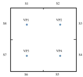
Figure 6 shows an example of how the data discretization works. The walls of the scanning scene are extracted from the 2D floor map and then discretized with a certain unit (e.g., segments with the length of 1m), as S1 to S8 in Figure 6. Similarly, possible viewpoints are also discretised as VP1 to VP4.
Figure 6. Example of the scanning problem
3.2 Scanning Geometry Constraints
As mentioned in Section 1, TLS observation quality is impacted by scanning geometry. Based on the existing research (Lichti, 2007; Pejic, 2013; Roca-Pardiñas et al., 2014; Soudarissanane et al, 2011), the observation quality is satisfactory when the scanner is placed where:
- The incidence angle of the laser beam is less than 60° - 65°; - The range between the object and the scanner is within the
range capability defined by the manufacturer.
These two factors are used as constraints in the network design. Since the test data is a small room within the range capability of most scanners, only the incidence angle constraint is considered in this paper. A Boolean score table for all discretised segments from an arbitrary viewpoint is obtained as Figure 7. The visibility zone for one viewpoint is the scanning area where the incidence angle constraint is satisfied. The marking rule is:
- Case 1: Two vertices of the segment fall into the visibility zone;
- Case 0: Less than two vertices of the segment is within the visibility zone.
Particle memory influence Swarm influence Particle motion influence
+
+ �
Initial Swarm with Particles , and
New Swarm with
, and
Termination Criteria
End Yes
No Update
Swarm Own Flying Memory
Swarm Influence
Optimal Particle and
Current flying
VP1 VP2
VP3 VP4
S1 S2
S6 S5
S3
S4 S8
S7
Figure 7. Boolean wall segments
The entire score table for the example in Figure 6 is constructed as Table 2.
Segments
VPs S1 S2 S3 S4 S5 S6 S7 S8
VP1 1 0 1 1 1 1 0 1
VP2 0 1 1 0 1 1 1 1
VP3 1 1 1 1 0 1 1 0
VP4 1 1 0 1 1 0 1 1
Table 2. Boolean score table for the example in Figure 6
3.3 Statement of Problem
It can be seen from Table 2 that the combination of any two and more possible VPs can provide a full coverage of the room. Furthermore, a quality measure needs to be determined for optimization. Since the observation quality is impacted by the incidence angle, the summation of all incidence angles of laser beams hitting the visible segment vertices is defined as the objective function in this optimization problem. A small sum of incidence angles corresponds to a network of good quality.
Finally, the optimization problem in this paper is stated as: determine the scanning network using heuristic methods to obtain a full coverage of the indoor scene with minimal number of scan locations as well as minimal summation of incidence angles.
4. APPLICATION
In this section, the SA, GA and PSO methods are used in the problem of optimizing an indoor TLS network design. Each
method’s performance is compared in terms of the quality of the solutions, runtime and repeatability. All methods are conducted on an Intel® CoreTM i5, 3.33GHz, 8 GB RAM computer, in the MATLAB R2015b environment.
4.1 Description
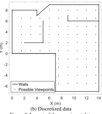
4.1.1 Experiment Environment: The experiment environment tested in this section is Room 125 in the CCIT building located on the University of Calgary campus. It has an area of 163.96 and is depicted in Figure 8(a).
(a) 2D floor map
(b) Discretized data
Figure 8. Layout of the experiment data
With the known coordinates of the room corners, the walls were extracted as shown in Figure 8(b). Using the method described in Subsection 3.1, the room was discretized into 74 wall segments with length of 1m and 68 possible viewpoints with an interval of 1.5m.
4.1.2 Pseudocode: Table 3 shows the pseudocode of the method used in the experiments. The room is discretized as wall segments S and possible viewpoints VP with their score tables ST. The method starts with one arbitrarily-selected viewpoint VP. The location of this viewpoint is updated using SA, GA or PSO and the summation of incidence angles the objective function. Another viewpoint is added into the viewpoints set VP if full coverage cannot be acquired with the current number of viewpoints. The method runs iteratively until a set of viewpoints with full coverage and minimum incidence angle summation is found.
Since the location of viewpoints generated by SA, GA and PSO can be any point bounded by the walls, it is time-consuming to construct a score table for each new viewpoint. To solve this problem, the nearest points of the newly-generated viewpoints are searched in VP. Then their corresponding score tables, which have been pre-generated, can be used directly to improve computation efficiency.
SA, GA and PSO in indoor network design
Input:S , = … , VP, ST , = …
Output: A set of viewpoints VP ∈ VP, = … , ≤ .
Initialization: VP , = whileVP , ≤
Update VP using SA, GA or PSO Search (the nearest VPin VP)
tempBest = Min (summation of the incidence angles) if ~full coverage
Add (one more viewpoint to VP , = + ) else
break end end
Table 3. Algorithm pseudocode Wall Segments
Viewpoint Visibility Zone
4.1.3 Parameters Selection: As shown in Table 4, different sets of empirical parameters were tested and their corresponding objective functions were used for evaluation.
Parameters #VP Objective
function°(×104)
SA
� = 104 °, � = 16m, � = 0.95 5 1.5670 � =102°, � = 16m, = 0.95 6 2.0677 = 104°, � =5m, = 0.95 6 1.9292 = 104°, � = 16m, �= 0.5 7 2.4493 GA
— 4 1.3328
PSO
� = 0.8, � = 0.1, � = 0.1 4 1.2536 = 0.1, = 0.8, = 0.1 5 1.4396 = 0.1, = 0.1, = 0.8 6 1.8069 = 0.33, = 0.33, = 0.33 5 1.5474
Maximum iteration: 3000
Number of chromosomes/particles: 30
Table 4. Parameters selection for each method
As can be seen In Table 4, the performance of each method varied with the selection of parameters. The maximum iterations for all methods was 3000 and the number of chromosomes or particles in GA and PSO was set to 30. No empirical values are required in GA. The parameters to provide optimal solutions for each method are listed in their first rows.
For SA, an extremely large initial temperature , an initial standard deviation � agrees with the room size and a slow cooling factor allow the candidate solutions to move widely within the moving area at first and eventually converge to the optimal solution. Parameters in its first row are proven to provide the optimal solution by varying a single parameter at a time. As in Table 4, tuning the parameters to other values prevents the SA method from finding optimal solutions.
For PSO, the optimal solution can be found when the inertial factor is much larger than and . By doing so the improvement to the solutions mainly depend on the randomly-generated movement, and are only slightly impacted by the current optimum. If the self-confidence factor or the swarm confidence factor is set larger, as in the second and third case in Table 4, the solution is more likely to be stuck in the current optima since the method trusts it too much. Tuning the factors to equal values provide a solution of the medium performance.
4.2 Results and Discussion
The performances of three adopted methods are compared regarding the quality of the solutions, runtime, and repeatability.
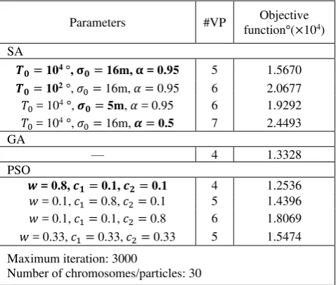
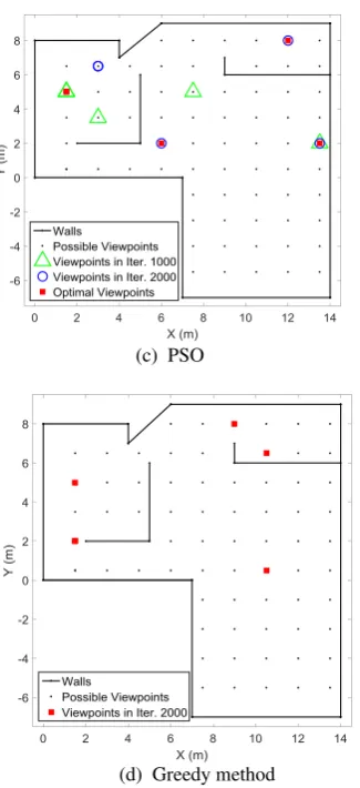
4.2.1 Quality of the Solutions: Successive solutions from the three heuristic methods as well as the greedy method are depicted in Figure 9. Represented by different symbols, the optimal solutions from iteration 1000, 2000 and 3000 are green triangles, blue circles and red squares, respectively. Their corresponding objective functions are also provided in Table 5.
It can be seen that within the maximum number of iterations, the performances of PSO and GA are similar. The optimal solution of PSO, i.e., 4 viewpoints with a minimum objective function of
1.2536×10⁴(°), can be found only when the parameter values are suitably selected, which is not an issue for GA. Since SA generates only one candidate per iteration, compared with 30 candidates in GA and PSO, it requires more iterations to find the optimal solution. Thus, SA cannot find a solution for 1000 iterations and only provides a solution with 5 viewpoints within the maximum number of iterations, which can be overcome when the iteration limitation is increased beyond 3000. The greedy method solution shows that a sub-optimal plan with a minimum of 5 viewpoints for this case can be obtained with no iteration, and the impact of being away from the optimum will increase in case of more complex scenes.
Iteration Successive solutions (Symbols in Figure 9)
Objective function °(×104) SA
1000 — —
2000 Blue circles (○) 1.7879
3000 Red squares (■) 1.5670
GA
1000 Green triangles (∆) 1.3416
2000 Blue circles (○) 1.3328
3000 Red squares (■) 1.3328
PSO
1000 Green triangles (∆) 1.3665
2000 Blue circles (○) 1.3276
3000 Red squares (■) 1.2536
Greedy method
Red squares (■) 1.7274 Table 5. Successive solutions and objective functions
(a) SA
(b) GA
(c) PSO
(d) Greedy method
Figure 9. Layout of optimal viewpoints from different methods
4.2.2 Runtime: Each optimization method was repeated 20 times and the average runtimes are listed in Table 6. GA and PSO have a similar total runtime and runtime per iteration. The reason that SA runs faster per iteration is because SA generates one solution once per iteration while other two methods generate 30 solutions in each iteration. However, since SA cannot find optimal solutions with 4 viewpoints, its total runtime is longer than the other two methods.
Method Ave. total runtime Ave. runtime per iteration
s s
SA 44.3436 0.0074
GA 37.4379 0.0125
PSO 35.5385 0.0118
Table 6. Average runtime
4.2.3 Repeatability: The objective functions for the solutions in 20 runs are used to evaluate the repeatability of each method. From Figure 10, one can see that solutions from GA and PSO are more repeatable than solutions from SA, which is demonstrated numerically in Table 7.
Method Mean Standard Deviation
°(×104) °(×102)
SA 1.7828 5.6039
GA 1.3688 1.7252
PSO 1.2784 1.4134
Table 7. Mean and Standard deviation of the objective functions
Figure 10. Objective functions in 20 runs
5. CONCLUSIONS
Compared with in geodesy and photogrammetry, optimal network design for TLS hasn’t received the same attention in current research. In this paper, the first-order design of an indoor TLS network, i.e., the configuration of scanner locations, is of interest. The experiment environment was simulated with discretized wall segments and possible viewpoints. A minimum number of viewpoints with a complete coverage of all wall segments was found by adopting three heuristic optimization methods: simulated annealing, genetic algorithm and particle swarm optimization. The experiment environment was a simulated room located on the University of Calgary campus.
Comparisons were made regarding the quality of the solutions, runtime, and repeatability. It was demonstrated that PSO has the best performance when its empirical parameters are selected suitably while SA performs the worst that cannot guarantee an optimal solution within the same iterations. GA provides similar solutions with PSO with tuning less empirical parameters. Thus, GA is determined as the best choice for this problem.
This problem is currently considered in 2D space, which can be further extended to the more complex 3D problems. Known as the Next Best View problem, this type of problem is normally solved by the strategy of ray-tracing, which is computational complex even for a trivial object (Pito, 1999). Also, constraints like the overlap rate between adjacent scans and the minimum range capability of the selected scanner can be involved. In addition, the number and configuration of targets is another consideration for optimal performance of point cloud registration. Eventually, a full design system that can automatically provide an optimal plan for the high-accuracy and large-volume scanning network is to be developed in this research.
REFERENCES
Abellán, A., Oppikofer, T., Jaboyedoff, M., Rosser, N. J., Lim, M., and Lato, M. J., 2014. Terrestrial laser scanning of rock slope instabilities. Earth surface processes and landforms, 39(1), pp. 80-97.
Asplund, L., 1963. Specifications for fundamental geodetic networks. Travaux de L'Association Internationale de Geodesie, 21, pp. 53-57.
Baselga, S., 2011. Second order design of geodetic networks by the simulated annealing method. Journal of Surveying Engineering, 137(4), pp. 167-173.
Becerik-Gerber, B., Jazizadeh, F., Kavulya, G., and Calis, G., 2011. Assessment of target types and layouts in 3D laser scanning for registration accuracy. Automation in Construction, 20(5), pp. 649-658.
Berné, J. L., and Baselga, S., 2004. First-order design of geodetic networks using the simulated annealing method. Journal of Geodesy, 78(1–2), pp. 47-54.
Boehler, W., Vicent, M. B., and Marbs, A., 2003. Investigating laser scanner accuracy. In: The International Archives of Photogrammetry, Remote Sensing and Spatial Information Sciences, XXXIV, Part 5, pp. 696-701.
Doma, M. I., and Sedeek, A. A., 2014. Comparison of PSO, GAs and analytical techniques in second-order design of deformation monitoring networks. Journal of Applied Geodesy, 8(1), pp. 21-30.
Fanti, R., Gigli, G., Lombardi, L., Tapete, D., and Canuti, P., 2013. Terrestrial laser scanning for rockfall stability analysis in the cultural heritage site of Pitigliano (Italy). Landslides, 10(4), pp. 409-420.
Gordon, S. J., and Lichti, D. D., 2004. Terrestrial laser scanners with a narrow field of view: the effect on 3D resection solutions. Survey Review, 37(292), pp. 448-468.
Grafarend, E. W., 1974. Optimization of geodetic networks. Bolletino Di Geodesia a Science Affini, 33(4), pp. 351-406.
Grossmann, I. E. (Ed.)., 2013. Global Optimization in engineering design, Springer Science and Business Media.
Holland, J. H., 1975. Adaptation in natural and artificial systems: an introductory analysis with applications to biology, control, and artificial intelligence. University of Michigan Press, Ann Arbor.
Hullo, J F., 2016. Fine registration of kilo-station networks - a modern procedure for terrestrial laser scanning data sets. In: International Archives of the Photogrammetry, Remote Sensing and Spatial Information Sciences, Prague, Czech Republic, Vol. XLI-B5, pp. 485-492.
Johnson, W. H., and Johnson, A. M. (2012). Operational considerations for terrestrial laser scanner use in highway construction applications. Journal of Surveying Engineering, 138(4), 214-222.
Kennedy, J., 2011. Particle swarm optimization. In: Encyclopedia of Machine Learning, pp. 760-766.
Kuang, S., 1996. Geodetic network analysis and optimal design: concepts and applications. Chelsea, Ann Arbor Press.
Lague, D., Brodu, N., and Leroux, J., 2013. Accurate 3D comparison of complex topography with terrestrial laser scanner: Application to the Rangitikei canyon (NZ). ISPRS Journal of Photogrammetry and Remote Sensing, 82, pp. 10-26.
Lichti, D. D., 2007. Error modelling, calibration and analysis of an AM--CW terrestrial laser scanner system. ISPRS Journal of Photogrammetry and Remote Sensing, 61(5), pp. 307-324.
Marmulla, R., Hassfeld, S., Lüth, T., and Mühling, J., 2003. Laser-scan-based navigation in cranio-maxillofacial surgery. Journal of Cranio-Maxillofacial Surgery, 31(5), pp. 267-277.
Metropolis, N., Rosenbluth, A. W., Rosenbluth, M. N., Teller, A. H., and Teller, E., 1953. Equation of state calculations by fast computing machines. The Journal of Chemical Physics, 21(6), pp. 1087-1092.
Mukupa, W., Roberts, G. W., Hancock, C. M., and Al-Manasir, K., 2016. A review of the use of terrestrial laser scanning application for change detection and deformation monitoring of structures. Survey Review, 49(353), pp. 99-116.
Oskouie, P., Becerik-Gerber, B., and Soibelman, L., 2016. Automated measurement of highway retaining wall displacements using terrestrial laser scanners. Automation in Construction, 65, pp. 86-101.
Pejić, M., 2013. Design and optimisation of laser scanning for tunnels geometry inspection. Tunnelling and Underground Space Technology, 37, pp. 199-206.
Pito, R., 1999. A solution to the next best view problem for automated surface acquisition. IEEE Transactions on Pattern Analysis and Machine Intelligence, 21(10), pp. 1016-1030.
Roca-Pardiñas, J., Argüelles-Fraga, R., de Asís López, F., and Ordóñez, C., 2014. Analysis of the influence of range and angle of incidence of terrestrial laser scanning measurements on tunnel inspection. Tunnelling and Underground Space Technology, 43, pp. 133-139.
Saleh, H. A., and Chelouah, R., 2004. The design of the global navigation satellite system surveying networks using genetic algorithms. Engineering Applications of Artificial Intelligence, 17(1), pp. 111-122.
Santagati, C., Inzerillo, L., and Di Paola, F., 2013. Image-based modeling techniques for architectural heritage 3D digitalization: limits and potentialities. In: International Archives of the Photogrammetry, Remote Sensing and Spatial Information Sciences, 5(w2), pp. 555-560.
Schmitt, G., 1982. Optimization of geodetic networks. Reviews of Geophysics, 20(4), pp. 877-884.
Schmitt, G., 1985a. Second Order Design. In: Optimization and Design of Geodetic Networks, Berlin, Heidelberg, pp. 74-121.
Schmitt, G., 1985b. Third order design. In: Optimization and Design of Geodetic Networks, Berlin, Heidelberg, pp. 122-131.
Son, H., Kim, C., and Kim, C., 2014. Fully automated as-built 3D pipeline extraction method from laser-scanned data based on curvature computation. Journal of Computing in Civil Engineering, 29(4), pp. 1- 9.
Soudarissanane, S., Lindenbergh, R., Menenti, M., and Teunissen, P., 2011. Scanning geometry: Influencing factor on the quality of terrestrial laser scanning points. ISPRS Journal of Photogrammetry and Remote Sensing, 66(4), pp. 389-399.
Soudarissanane, S., Lindenbergh, R., 2011. Optimizing terrestrial laser scanning measurement set-up. In: ISPRS Laser Scanning 2011, Calgary, Vol. XXXVIII, pp. 1-6.
Wujanz, D., & Neitzel, F., 2016. Model based viewpoint planning for terrestrial laser scanning from an economic perspective. In: International Archives of the Photogrammetry, Remote Sensing and Spatial Information Sciences, XLI(B5), pp. 607-614.
Ye, C., and Borenstein, J., 2002. Characterization of a 2-D laser scanner for mobile robot obstacle negotiation. In: 2002 IEEE International Conference on Robotics and Automation, Washington DC, USA, pp. 2512-2518.