A model to estimate the temperature of a maize apex from
meteorological data
Lydie Guilioni
a, Pierre Cellier
b,∗, Françoise Ruget
c, Bernard Nicoullaud
d,
Raymond Bonhomme
baLaboratoire d’ Ecophysiologie des Plantes sous Stress Environnementaux, INRA-AGRO.M, UFR Agronomie et Bioclimatologie, 2, place
Viala, 34060 Montpellier Cedex 02, France
bINRA, Unité de Recherche en Bioclimatologie, F78850 Thiverval-Grignon, France cINRA, Unité de Recherche en Bioclimatologie, 84914 Avignon Cedex 9, France dINRA, Service d’Etude des Sols et de la Carte Pédologique de France, Ardon, 45160 Olivet, France
Received 16 September 1998; received in revised form 23 July 1999; accepted 17 September 1999
Abstract
During early growth, when the apical meristem of a maize plant is close to the soil surface, its temperature may be very different from air temperature. A model is proposed to estimate apex temperature from meteorological data, when the leaf area index is less than 0.5. This model is based on the energy balance of the apical meristem, considered as a vertical cylinder close to the soil surface, called ‘apex’. Soil surface temperature was calculated from an energy and water balance of the soil. Input data were hourly standard meteorological data and soil texture. Stomatal conductance was calculated from solar radiation and water vapor deficit.
Five field experiments with different soil and climatic conditions were conducted to calibrate and validate the model. The roughness length of the soil surface was used as a calibrating factor. The selected value was 0.3 mm, and was used on all datasets. The agreement between observed and calculated apex temperatures was fairly good, with residual standard deviations between 0.8 and 1.9 K in five experiments, while apex temperature was generally higher than air temperature at screen level by more than 5–7 K during the day. This study showed that the main problem to overcome in estimating apex temperature, is to calculate air temperature at apex height, i.e. at several centimeters from the soil surface. This requires development of precise soil surface temperature models. ©2000 Elsevier Science B.V. All rights reserved.
Keywords: Maize; Meristematic zone; Temperature; Prediction; Energy balance; Meteorological data
1. Introduction
Temperature has a major influence on plant growth and particularly on development rates. Many studies have shown that leaf initiation, leaf appearance and elongation are strongly related to temperature (Watts,
∗Corresponding author. Tel.:+33-1-30-81-55-55;
fax:+33-1-30-81-55-63.
E-mail address: [email protected] (P. Cellier).
1972a; Warrington and Kanemasu, 1983 in maize; Gallagher, 1979 in wheat and barley; Ong, 1983 in pearl millet). De Reaumur first suggested in 1735 (De Reaumur, 1735) that the duration of particular stages of growth was directly related to temperature and that this duration for a particular species could be pre-dicted using the sum of mean daily air temperature. This way of normalizing time with temperature, the thermal time, in order to predict the plant development rates has been widely used in this century (Durand
et al., 1982; Ritchie and NeSmith, 1991). The concept of thermal time assumes a strong correlation between air temperature and that sensed by the plant (Durand et al., 1982). But in maize, like in many monocot crop plants, the specific locations where temperature influ-ences development — i.e. the zones where cell divi-sion and expandivi-sion are occurring (Kleinendorst and Brouwer, 1970; Watts, 1972b; Peacock, 1975) — are close to the soil surface during early growth. In these conditions, the development rates (leaf initiation, leaf appearance or reproductive initiation rate) are not ac-curately related to air temperature (Beauchamp and Lathwell, 1966; Brouwer et al., 1970; Aston, 1987). Duburcq et al. (1983) have shown that the develop-ment rate of maize until male floral initiation was bet-ter related to soil temperature than to air temperature. Swan et al. (1987) found that the development rate of maize was best described using soil temperature until the sixth leaf was fully developed. More recently, Shar-ratt (1991) over barley and Bollero et al. (1996) over maize observed different development rates under dif-ferent controlled soil temperatures. Moreover, looking directly at plant temperature, either in growth-chamber or in field conditions, Ben Haj Salah and Tardieu (1996) observed that leaf elongation rate was corre-lated better with meristematic apex temperature than with air temperature. Similarly, Jamieson et al. (1995) calculated thermal time based on plant temperature. They concluded that ‘a model of leaf appearance based on near surface temperature and canopy temperature gave superior prediction than others based on air tem-perature’.
Cellier et al. (1993) have shown that the tempera-ture of the meristem was significantly different from both air and soil surface temperatures. The differences between air temperature at screen height and meris-tem meris-temperature reached almost 6 K for a daytime average, which means that hourly values were much larger. Thus, accounting for the influence of tempera-ture on growth and development should be improved by using the actual temperature of the extension zones. Beauchamp and Torrance (1969) proposed a model for estimating the internal temperature of a young maize plant. The maize stem was represented as a vertical cylindrical bar with one end in the soil considered as an infinite source of heat. This model overestimated the temperature of the plant certainly because neither the circulation of water in the stem nor the
transpi-ration was considered. Cellier et al. (1993) proposed a model — based on a energy balance equation — to predict the differences between air and meristem temperatures from standard meteorological data dur-ing the early growth of a maize plant. However, this model presented some limits. The radiation balance neglected the shade of leaves, and in the absence of any references, the stomatal conductance of the meris-tematic zones was a fitting parameter. Furthermore, the output data are averages of day and night temperatures with no way to estimate maximum or minimum which may be the most relevant temperatures for explaining differences in development rate (Weaich et al., 1996). In this paper, we proposed a model based also on an energy balance approach, for estimating the temper-ature of the extension zones of a young maize. This model works at hourly time steps, from standard me-teorological data. The main improvements compared to the original model of Cellier et al. (1993) are related to the radiation balance, the stomatal conductance pa-rameterization and the air temperature profile near the soil surface.
2. Methods
2.1. Model
The extension zones (consisting of both leaves and apical meristem) which are often called ‘pseudo-stem’, will be referred to as ‘apex’ in the following text. The apex temperature, denoted Tm, is calculated from the
During daylight, the main energy input to the apex is radiation, both solar and long-wave radiation. A part of this energy is released by evaporation through stomata. If apex temperature is different from air temperature at the same height, energy may be absorbed or released as sensible heat by convection. Moreover, energy may be transferred through the apex in a vertical direction by convection and/or conduction. During the night, most of these fluxes change sign. The radiation balance is negative, and water vapor may condense on the apex.
The energy balance of the apex can be written
Rnm+Gm+Hm+λEm=0 (1)
where Rnm is the net radiation, Hm andλEm are the
sensible heat and the latent heat fluxes between the apex and the surrounding air. Gm is the transport
of heat along the apex by conduction through the plant tissues or convection by sap flow. The values of the parameters mentioned in the following equa-tions are summarized in Table 1, and the notaequa-tions are recapitulated in Appendix A. All the input data of the model are (1) data measured by a standard meteorological station and (2) plant characteristics with fixed values. The model calculates apex tem-perature over short time steps (1 h or less). It is the only time step for which the hypothesis of stationarity of the energy balance and several parameterizations such as that of stomatal conductance or temperature profiles (see below) are valid. This model runs in the early growth stages, when leaf area index (LAI) is less than 0.5 m2m−2. This limitation is imposed by the parameterization of both radiative and con-vective schemes. With taller crops a more complex
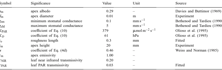
Table 1
Values and origin of the constants used in the model
Symbol Significance Value Unit Source
am apex albedo 0.29 – Davies and Buttimor (1969)
dm apex diameter 0.01 m Experiment
gsm minimum stomatal conductance 0.1 mm s−1 Bethenod and Tardieu (1990)
gsM maximum stomatal conductance 5 mm s−1 Bethenod and Tardieu (1990)
KPAR coefficient of Eq. (10) 379 mmol m−2s−1 Olioso et al. (1995)
KD coefficient of Eq. (10) 61 hPa Olioso et al. (1995)
zo roughness length 0.3 mm Fitted
zm apex height 20 mm Experiment
α coefficient of Eq. (4d) 0.46 – Weiss and Norman (1985)
εm apex emissivity 1.00 –
τNIR leaf near infrared transmissivity 0.20 –
τPAR leaf PAR transmissivity 0.03 – Fitted
ear, pea flower, top leaves) the temperature difference should be much larger, especially in the case of a non-evaporating organ (e.g. a bud before bud burst). On the other hand, the temperature difference between the air at screen height and the air surrounding the apex (first step) can also be very variable according to the field conditions: from several degrees or tens of degrees over a bare dry soil (Garratt, 1988; Cellier et al., 1996) to several tenths of degrees over an evap-orating vegetation or a wet soil. Consequently, both temperature differences must be considered to build a model adapted to a wide range of vegetation and me-teorological conditions and to be able to analyze what determines plant temperature.
2.1.1. Temperature and wind speed profiles above the soil surface
Due to interactions between free and forced convec-tion air temperature and wind speed profiles cannot be determined independently from each other. Moreover, both air temperature Tam, and wind speed, Um, at apex
height are required in some fluxes of the energy bal-ance equation. Wind speed and air temperature varia-tion with height are generally described by using the flux-gradient relationships given by Dyer and Hicks (1970)
where u(z) and T(z) are the wind speed and air temper-ature at height z; u∗is friction velocity, T∗a scale
tem-perature, and zoand zoh are the roughness lengths for
momentum and heat transfer. As generally assumed,
zoh was taken equal to 0.1zo (Brutsaert, 1982). The
Monin–Obukhov length, L, is related to u∗and T∗by
L=T/kg u2∗/T∗. The stability functions9M and9H
account for the effects of vertical temperature gradient on convective transfer (Dyer and Hicks, 1970). Their expressions were derived by Paulson (1970).
Determining the wind and temperature profiles re-quires calculation of u∗, T∗ and L using Eq. (3) and
analogous equations. For this, the air temperature at
zoh, To, must be determined. This was done using an
energy balance of the soil surface, including a soil sur-face water balance as described in Appendix B. This
method makes it possible to account for the variations of soil surface temperature due to meteorological con-ditions and soil wetting/drying according to the cli-matic factors and capillary water transfer in the top soil. The height where Tam and Umare calculated as
that of the apex, zm was taken as 0.02 m.
2.1.2. Radiation balance
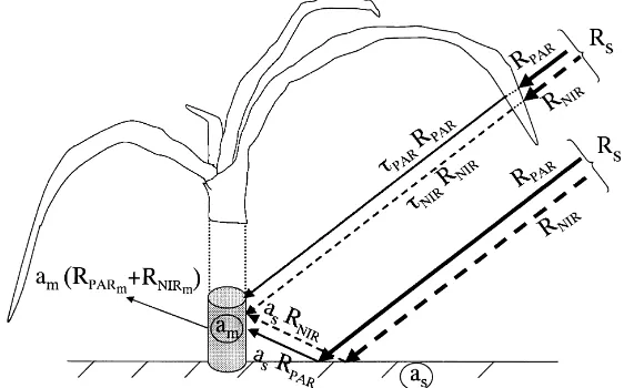
The radiation balance is divided into short-wave and long-wave radiation balances. Visual observation showed that for most of the day, the apex was shad-owed by its own leaves or those of the neighbouring plants in the same row. This is especially true when the solar elevation is high, i.e. when solar radiation is at this peak. We could then consider that short-wave radi-ation reaching the apex was either transmitted through the leaves or reflected from the soil (Fig. 1). In both cases, it is diffuse radiation. As leaf transmittance is different for photosynthetically active (PAR) and near infrared radiation (NIR), these spectral intervals have to be considered separately. Moreover, PAR radiation is required for calculating stomatal conductance (see below). Due to shadowing by leaves, no directional ef-fect of radiation was considered. Short-wave radiation balance, RSWm, may then be expressed as
RSWm=(1−am)(RPARm+RNIRm) (4a)
with
RPARm=(τPAR+as)RPAR (4b)
and
RNIRm =(τNIR+as)RNIR (4c)
where am and as are the plant and soil albedos. Also
τPARandτNIRare the transmittances of leaves in the
PAR and near infrared wavelength ranges. RPAR and
RNIR are the PAR and NIR inputs over the canopy
obtained from the solar radiation Rs by
RPAR=αRs (4d)
RNIR=(1−α)Rs (4e)
Following Weiss and Norman (1985),αwas taken equal to 0.46. All radiation components are expressed in units of W m−2. In RPARmand RNIRmthe index ‘m’
Fig. 1. Schematic representation of the short-wave radiation balance of the apex (Rs, solar radiation; RPAR, RNIRincident PAR and incident NIR above the crop; RPARm, RNIRm, PAR and NIR at the apex surface; amapex albedo; assoil albedo;τPAR,τNIR, leaf transmissivity for PAR and NIR).
The long-wave radiation balance is written
RLWm=εm(Ram−σ Tm4) (5)
The first term on the right-hand-side of Eq. (5), Ram,
is the long-wave radiation input from the surround-ing environment (sky, leaves, soil). This flux was ex-pressed as
Ram =
σ Ta4+σ Ts4
2 (6)
where Ta is air temperature (K) measured at screen
height and Tsis the soil surface temperature. The first
term on the right-hand side of Eq. (6) isσ Ta4instead of atmospheric radiation because it can be considered that the apex mainly ‘looks at’ the lower atmosphere at large angles from the zenith and maize leaves (whose temperature is close to air at screen height) at low angles (Fig. 1). The second term in the right-hand-side of Eq. (5) represents the long-wave radiation losses linked to the apex temperature. The apex emissivity,
εm, is taken equal to 1.00, as usually done for most
vegetation, and the soil emissivity too.
2.1.3. Sensible heat exchanges
The transfer of sensible heat from the apex to the surrounding air is considered as proportional to the temperature difference between the apex and the air at apex height
Hm=ρcpgm(Tm−Tam) (7)
where Tamis air temperature at apex height, and gmis
a thermal diffusion conductance. Its value depends on the wind speed at apex height, Um, and on the apex
diameter, dm. It can be expressed according to the
expression given by Finnigan and Raupach (1987).
gm=0.54
U
m
dm 1/2
(8)
Tamand Umwere calculated from air temperature and
wind speed profiles as previously described.
2.1.4. Evaporation
The transpiration from the apex is mainly regulated by stomata. It may be expressed in a form similar to that of the sensible heat flux,
λEm=
ρcp
γ
em−eam
1/gv+1/gs
(9)
where eam is the vapor pressure at apex height and
emis the vapor pressure inside substomatal chambers
of the leaves which constitute the external face of the apex. It is taken equal to the saturation vapor pres-sure at apex temperature; eam can be calculated from
procedure described in Appendix B; gv is a thermal
diffusion conductance, equal to 0.89gm(Eq. (8)).
The stomatal conductance, gs, is controlled by
dif-ferent environmental factors, among which radiation, water vapor pressure deficit, soil water content and at-mospheric carbon dioxide concentration are the most important (Jarvis, 1976). Considering that, just after sowing, soil water content was rarely a limiting factor,
gs was modeled using only a regulation by solar
ra-diation and water vapor deficit. The relation proposed by Olioso et al. (1995) was used,
gs=gsm+(gsM−gsm)
where gsm and gsMare the minimum and maximum
conductances (m s−1), D is the water vapor pressure air deficit at apex level; QPARis RPARm (Eq. (4)), but
expressed inmmol m−2s−1; KPARand KDare constant
coefficients given by Olioso et al. (1995) (see Table 1).
2.1.5. Heat flux through the stem
Under daytime conditions, heat is transported from the underlying warmer ground to the leaves by sap flow through the apex. Temperature measurements be-low and above the apex showed that the amount of heat transported by this way was less than 10% of the net radiation in all cases, and their difference, which represents the energy storage by the apex was much less. Therefore, this flux was neglected.
2.1.6. Calculation of the apex temperature
Using Eqs. (1) and (4)–(10), the energy balance equation was solved at each time step using an itera-tive procedure. The iteration of apex temperature was terminated when the energy balance closed to within 1 W m−2. The same approach was used at the same time to calculate soil surface temperature and water content, using Eqs. (B.1)–(B.10). If not available, the soil water content was initialized to 75% of the field capacity for the surface layer, and to the field capacity for the deep soil layer. The apex temperatures calcu-lated during the first day were excluded from the anal-ysis so that the results might not be affected by badly estimated initial soil water contents.
2.2. Field experiments
2.2.1. Field conditions
This model was calibrated and tested with five datasets, collected at three sites. Three experiments were conducted in Grignon, France (48◦51′N, 1◦58′E, altitude 125 m), one in 1990 and two in 1993, over a 1.4 ha maize field (Zea mays L.) of the INRA ex-perimental station, with a clay-loam soil. The albedo was 0.20 under dry conditions, and decreased to 0.15 after rainfall. In 1990, the maize was sown on 4 May (day of year (DOY) 124) and the measurements of apex temperatures were made from 23 May (DOY 143) to 30 May (DOY 150). In 1993, two sub-plots of 40 m×40 m (called A and B) were sown in the same field at two different dates in order to get different cli-matic conditions, especially temperature. The maize was sown on 7 May 1993 on plot A and on 9 June on plot B. Apex temperatures were measured from 15 to 29 June for A and from 4 to 15 July for B. The three experiments performed in Grignon will be referred to as Grignon90, Grignon93A, and Grignon93B.
Two other experiments were conducted in 1992 in two farmers’ fields near Pithiviers, France (48◦08′N, 2◦13′E, altitude 120 m). The first (called ‘Brosses’) was on a calcareous loamy soil with small stones and the second (called ‘Lacour’) was on a loamy sand soil. The apex temperatures were measured from 22 to 29 May. Over both fields, the albedo was 0.30 when the soil surface was dry. After raining, it decreased to 0.20 at Lacour and 0.15 at Brosses.
In all experiments the maize variety was DEA, and the plant density was about 90,000 plants ha−1. During all experimental periods, the maximum crop height was between 0.1 and 0.4 m.
2.2.2. Micrometeorological measurements
In all experiments, the following measurements were made: (1) total downward solar radiation flux density on a horizontal surface (Rs), with a CM6
in the others), (4) air relative humidity at 2 m with a HMP35 capacitive hygrometer (Vaisala, Helsinki, Finland), (5) apex temperatures using thermocouples (AWG30) inserted into the plant, with a variable num-ber of replications according to the experiment (six in
Grignon90, nine in Grignon93, and four in Brosses
and Lacour). The thermocouples were inserted at heights between the soil surface and a height of 3 cm. Additional measurements were made during the Grignon experiments. Soil surface temperature was measured, using six copper–constantan thermocou-ples fixed on the soil surface with a thin plastic stem. The sensors were previously coated with a thin layer of mud in order to have optical properties similar to the soil. In Grignon93B, the photosynthetic active ra-diation received by the apex was measured using five photovoltaic amorphous silicon cells (Chartier et al., 1989) (SOLEMS, Palaiseau, France) put vertically near the apex, two of them facing north, the three others facing, respectively, south, east and west. The PAR reaching the apex was estimated as the aver-age of these five measurements, the two facing north being averaged to give one single value.
All these data were collected every 10 s on a dat-alogger (Campbell Scientific, Shepshed, UK) and av-eraged over 30 min.
2.2.3. Stomatal conductance
Many studies have been published on the stomatal conductance of maize leaves but, to our knowledge, no reference was available on the conductance of the sheath of maize leaves, or of such a system as the apex, made of rolled leaves, whose external face is composed of the sheaths of leaves. Therefore, obser-vations were made in order to (i) check if stomata were present at the apex surface, (ii) estimate their density, and (iii) get some values of stomatal conduc-tance of the apex, in order to integrate minimum (gsm)
and maximum (gsM) values in Eq. (10).
The stomatal density (number of stomata per mm2) was determined on the sheath or on the limb by press-ing small pieces of sheath or limb onto a rhodo¨ıd® plate softened with acetone (Schoch and Silvy, 1978). The prints of leaf epidermis, were observed under a microscope (amplification of 125). The stomatal den-sity of ten leaves was determined in ten different parts of the same print.
The stomatal conductance of the apex was measured with a LI-700 porometer (LI-COR, Lincoln, Nebraska, USA), by applying the measurement chamber on the sheath of the first leaves, between 0 and 5 cm above the soil surface. Measurements were made on several days, at different times of the day with various solar radiation densities. During two clear days, we related
gs to the PAR received by the apex. Each stomatal
conductance measurement was coupled with a mea-surement of the PAR, using a photovoltaic amorphous silicon cell (Chartier et al., 1989) put vertically near the apex.
3. Results
3.1. Experimental results
3.1.1. Observed apex temperatures
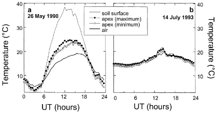
We compared the range of observed apex temper-atures with air and soil surface tempertemper-atures for two days with different meteorological conditions during
Grignon90 and Grignon93 experiments (Fig. 2). Solar
radiation was high (28.2 MJ m−2 for the day) on 26 May 1990 at Grignon (Fig. 2a), and it was much less on 14 July 1993 (7.7 MJ m−2, Fig. 2b). As solar radi-ation was high on Fig. 2a, the soil surface temperature became much higher than air temperature, and conse-quently air temperature at apex height and apex tem-perature increased, too. The temtem-perature differences between air and soil surface and between air and apex reached 21.3 and 7.3 K, respectively. These differences were not exceptional: over the five datasets mentioned
above representing 48 days of measurements, the max-imum temperature difference between the apex and air at 2 m was more than 10 K for 4 days, 7 K for 21 days and 5 K for 35 days. It was less than 4 K for only 5 days. Apex temperatures were also higher than air tem-perature during an overcast day (Fig. 2b). Even with low solar radiation, the apex temperature was clearly different from air temperature at screen height. The difference was larger than 2 K near midday.
Compared to the difference between apex and air temperature, the variability of apex temperatures, es-timated from the replicates, was low. The largest am-plitude was less than 2 K, which is much less than the difference with air temperature. This will allow us to consider only the average apex temperature for testing and validating the model.
3.1.2. Stomatal conductance
Visual observations showed the presence of stomata on the leaf limb, but also on the external face of the sheath. However, the stomatal density was lower on the sheath (28±12 stomata mm−2) than on the leaf limb (98±20 on the lower face and 51±18 on the up-per face). Stomatal conductance measurements were made over a wide range of radiation, from 0 to more than 1400mmol m−2s−1. At any radiation, low
stom-atal conductances were observed (less than 5 mm s−1). The maximum values were observed for radiations above 800mmol m−2s−1. The large variability in Fig.
3 has been classically observed in many previous stud-ies (see, e.g., Jones (1992) and Bethenod and Tardieu (1990)). It may be due to either other limiting factors (soil water potential, vapor pressure deficit) or due to a technical problem such as leaks when using the dif-fusion porometer, which is not adapted to the shape of the apex (Turner, 1991). However, despite the lower stomatal density, the change in stomatal conductance with radiation and the maximum values were similar to previously published values. Thus, we considered that the apex behaved like a leaf, and we chose for the maximum stomatal conductance in Eq. (10) the values given by Bethenod and Tardieu (1990) (see Table 1).
3.1.3. PAR reaching the apex
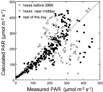
In Fig. 4 are compared the PAR balance of the apex measured using the five silicium cells and that esti-mated using Eqs. (4b) and (4d), for 11 days during
Fig. 3. Stomatal conductance estimated with a diffusion porometer as a function of PAR near the apex. The curve is the relation between PAR and stomatal conductance as expressed by Eq. (10), excluding the vapor pressure deficit effect (D=0).
Grignon93B. The best fit between measured and
cal-culated values was obtained with a PAR transmissivity of 0.03. This value forτPAR is consistent with most
published values, which range from 0.01 to 0.05. The global trend is around the 1 : 1 line, but with large dispersion at high values. Most values underestimated by Eq. (4b) came from data collected early in the morning, when direct solar radiation reaches the apex, which is not accounted for in the model. These data,
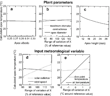
Fig. 5. Sensitivity of the model to the plant parameters: (a) apex albedo, (b) apex diameter and maximum stomatal conductance, (c) apex height above the soil surface and to the forcing variables, (d) solar radiation and wind speed and (e) air and dew point temperature.
corresponding to hours before 9 a.m., are plotted with crosses. On the contrary, PAR calculated near mid-day overestimated the measurements because a larger fraction of the soil is shadowed by the leaves of the maize canopy, and consequently the reflected PAR is certainly less than assumed in Eq. (4b). These data are represented as open circles in Fig. 4. Despite these limitations, the comparison was considered as satisfac-tory for our application, with such simple input data.
3.2. Sensitivity study
The sensitivity of the model to either the forcing variables, i.e. the input meteorological data, or to the plant parameters (albedo, diameter, maximum stom-atal conductance and apex height) was analyzed. The model was run using the parameters given in Table 1, by changing only one variable or parameter by more than twice the uncertainty on it. The chosen ranges
of variation were±20% for solar radiation and wind speed,±2 K for air and dew point temperature,±50% for maximum stomatal conductance and apex diame-ter,±10 mm for apex height and±0.05 for albedo. The average values given in Table 1 are either taken from the scientific literature or fitted to our experimental data (see next section). The input meteorological data are those from the Grignon90 experiment which, were also used for calibrating the model (see next Section). They come from fine weather days with high solar ra-diation and large temperature differences between the apex and air. Under such conditions, the effect of any parameter or variable should be most evident. The re-sults are plotted in Fig. 5a–e.
Finally, the only plant parameter to which the model is sensitive, is the apex height. This is the conse-quence of the steep air temperature variation with height near the soil surface.
For the meteorological variables (Fig. 5d–e), the sensitivity is larger. It remains low for the dew point temperature. It is slightly larger for wind speed. The sensitivity to solar radiation is large (±0.8 K for a change in solar radiation of 20%), but the calculated apex temperature is most sensitive to the air tempera-ture (±1.8 K for a change in air temperature of±2 K).
3.3. Model calibration
The sources of uncertainty in this model can be classified as relative to either the local energy balance of the apex, or to the way of estimating the micro-climatic variables at apex height. Most parameters in the local energy balance could be directly determined (size, soil albedo), or chosen from the literature (apex albedo, emissivity, maximum stomatal conductance) (Table 1). Moreover, the sensitivity study showed that the calculated apex temperature was not very sensi-tive to these parameters, but was very sensisensi-tive to air temperature.
Consequently, the air temperature at apex height must be determined as precisely as possible. For this, the main parameter to know is the roughness length (Eq. (2)). However, it is not possible to use an aero-dynamic roughness length directly estimated from the physical characteristics of the soil surface and the maize crop, using simple relations with the physi-cal surface roughness (height of obstacles; . . .) for two reasons. First, the logarithmic wind and temper-ature profiles cannot be extended down to the apex height, because the flux-gradient relationships are not strictly valid at low z/zoratios (Tennekes, 1973;
Cel-lier and Brunet, 1992). Secondly, it is not straight-forward to derive one roughness height for the whole wind and temperature profile from the reference height to the soil surface, when two flows should be con-sidered: one above the canopy and another near the soil surface (the maize crop was generally taller than 0.3–0.4 m when the LAI reached 0.5). Thus, as it could not be determined a priori, the roughness length was used as a fitting parameter for the model. For the rea-sons expressed above, it could not be considered as
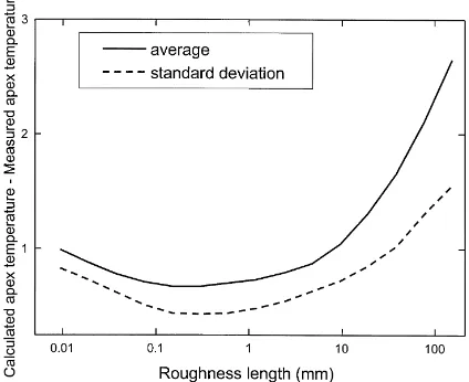
Fig. 6. Roughness length dependence of the average and of the standard deviation of the absolute value of the difference between calculated and measured apex temperatures. The input data are those from the Grignon90 experiment.
a realistic roughness length but only as a way to re-late air temperature at apex height to air temperature at screen height. Classical flux-gradient relationships (Eqs. (2)–(3)) were used in order to account for the in-fluence of the surface energy balance and the turbulent flow characteristics on the temperature profile. Using the Grignon90 experiment, the roughness length giv-ing the best fit between calculated and observed apex temperatures was determined. The observed temper-ature was taken as the average of the six apex tem-peratures measured in this experiment. In Fig. 6 are plotted the average and the standard deviation of the absolute value of the difference between calculated and measured apex temperatures. Both curves show an optimum for roughness lengths between 0.2 and 0.6 mm, with a minimum value at 0.3 mm. Thus, a roughness length of 0.3 mm was chosen. It is much less than the roughness length that could have been determined from the crop height and leaf area den-sity, i.e. 10–40 mm. This confirms that this roughness length is nothing more than a fitting parameter.
On Fig. 7 are presented the observed and calculated apex temperatures during the Grignon90 experiment (with zo=0.3 mm). It can be seen that the model gives
Fig. 7. Air temperature, measured and calculated apex temperature during the Grignon90 experiment.
is important because it is during fine weather days that the temperature difference between apex and air is at its largest. The gradual temperature decrease in the night and the minimum are also well simulated, even though the energy transfer processes are very different during day and night.
3.4. Model validation with other datasets
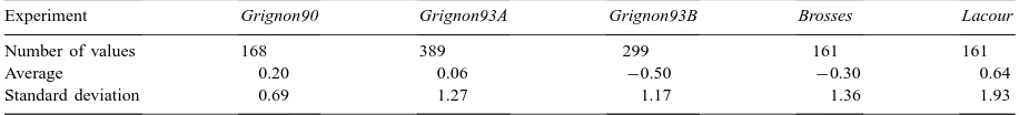
The model with the roughness length determined over the Grignon90 experiment has been applied to the other independent datasets presented previously. This comparison was made only on the daytime period, between sunrise and sunset, because this is the pe-riod when the temperature differences are the largest. Moreover, it is often biased to compare averages cal-culated over a 24 h period, because the energy transfer processes are opposite between day and night. Thus, a bad account of energy transfers could give the same average, while the temperature may be underestimated during day and overestimated during night, or the re-verse. The results are given in Fig. 8 and Table 2. The averages and dispersion are larger on these
experi-Table 2
Average and standard deviation (K) of the difference between observed and calculated apex temperature during the day (Rs≥50 W m−2)
Experiment Grignon90 Grignon93A Grignon93B Brosses Lacour
Number of values 168 389 299 161 161
Average 0.20 0.06 −0.50 −0.30 0.64
Standard deviation 0.69 1.27 1.17 1.36 1.93
Fig. 8. Comparison of half hourly values of calculated and measured temperature difference between the apex and air at screen level, for (a) Lacour, (b) Brosses, (c) Grignon93A and (d)
Grignon93B experiments.
ments than on Grignon90. This is, of course, partly be-cause the model was calibrated with Grignon90 data, but also because the weather was much more chang-ing over these experiments, with frequent rainfall and changes in solar radiation, which induced a great vari-ability in air and soil surface temperatures.
4. Discussion
be 5–10 K warmer during day and 2–3 K lower during night in the case of a cloudless day. Therefore, the re-lation between apex temperature and air temperature in a meteorological station is not straightforward. It may be different both for average and extreme tem-peratures. This difference should be considered when analyzing the response of a maize crop to either high temperatures — which may diminish photosynthesis — or low temperatures (frost). Due to the asymmetry of the temperature difference, the daily average (over 24 h) of apex temperature is larger than that of air temperature. The difference ranged from 0 to 2 K on our experimental datasets. Such differences may have strong implications for accounting for the effects of temperature on growth and development.
The model that is presented in this paper should al-low replacement of air temperature by an apex tem-perature in crop models, or for estimating the risk of climatic stress (frost, heat stress). It is particularly adapted for operational application since (1) it uses only standard meteorological data and (2) some impre-cision in the plant parameters is permitted, because the sensitivity study showed that the model was insensi-tive to the plant parameters. The good agreement after fitting between calculated and measured apex temper-ature at any time in the day on the Grignon90 dataset showed that the energy balance approach was well adapted to this application. The model behaved fairly well under both daytime and night-time conditions, which are very different from an energy balance point of view: stable atmospheric conditions, no evaporation and a radiation deficit occur during the night, while daytime is characterized by a high radiation input, evaporation regulated by stomata, larger wind speed, and very large soil surface temperatures. In particular, the fair agreement between calculated and measured apex temperature near sunset and sunrise, when tem-perature changes rapidly, shows that the hypothesis of stationarity of the energy balance over the considered time step (30 min) was reasonable. This allows one to estimate with a good accuracy the average, minimum, and maximum temperatures.
Such a model also helps in interpreting apex tem-perature and factors that determine it. A surprising result was the low sensitivity of the model to stomatal conductance. This is mainly because evaporation is a minor term of the energy balance in the case of a maize apex. In fact, due to shading by leaves, and to the low
transmittance of the leaves for PAR, the stomatal con-ductance was low and the evaporation, too. The tem-perature is then mainly determined by an equilibrium between net radiation, Rnm, and sensible heat flux,
Hm, which is large for small temperature differences.
Over the Grignon90 dataset, the calculated sensible heat flux was approximately proportional to the calculated temperature difference between the apex and the air at apex height, with a slope of 220 W m−2K−1. Net radiation was always less than
250 W m−2. An uncertainty of ±50% on apex tran-spiration — which would result in a flux error of approximately 50 W m−2 as calculated by the model on the Grignon90 data — would be compensated by a variation in Hm with a change of 0.2 K in apex
temperature. Another result of the sensitivity study, was the relatively low response of apex temperature to solar radiation (0.8 K for a change in solar ra-diation of ±20%). This may also be explained by the high aerodynamic conductance of the apex, but also by the change in stomatal conductance. The PAR radiation reaching the apex was always low (<500mmol m−2s−1), a level where stomatal
conduc-tance is still increasing with increasing PAR (see Fig. 3). Thus, any increase in solar radiation was partly compensated by an increase in evaporation, which makes the apex temperature generally close to the air temperature at the same height. The calculated tem-perature differences between the apex and air at the same height on the Grignon90 dataset were always less than 0.8 K, whereas the temperature difference between the air at the apex height (2 cm above soil surface) and air at the reference height (2 m) often reached 6 K near midday.
Finally, it can be concluded that the lack of knowl-edge about the energy exchange parameters of a maize apex is not a great problem for estimating apex temper-ature because it is not very sensitive to most plant pa-rameters. This is mainly because (i) the apex receives a low amount of radiation due to the overlying leaves protecting it from direct solar radiation, (ii) a sig-nificant fraction of this radiative energy is consumed by evaporation, which transforms energy at constant temperature and (iii) the small aerodynamic resistance makes the sensible heat flux increase rapidly when the apex temperature goes above air temperature.
energy balance module is not strictly necessary to esti-mate apex temperature under such conditions. In order to check this, the model was run in a simplified ver-sion by considering that apex temperature was equal to air temperature at the same height. The model then only consisted in the soil surface energy balance pre-sented in Appendix A. As previously done for the complete model the surface roughness length was fit-ted on the Grignon90 dataset. The best value is close to the previous one: 0.35 mm instead of 0.30 mm. How-ever, both the absolute error and the residual stan-dard deviation are larger by approximately 0.1 K, i.e. 10–15 and 15–20%, respectively, with this simpler model compared with the initial model. Using a rough-ness length based on the canopy physical description, i.e. values comprised between 10 and 40 mm leads to much worse results. Both the absolute error and the residual standard deviation are multiplied by more than 2. Moreover, it must be emphasized that using only the soil surface energy balance model produces a simplification only by reducing the number of equa-tions. The input meteorological variables, which are the key-point for deciding whether a model is opera-tional or not, are the same for both models. The com-plete model has the advantage of being more general and easily adaptable for calculating the range of apex temperature (i.e. shaded and sunlit apex) or the tem-perature of any plant organ. For example, for an or-gan placed near the top of the crop (leaf, flower, ear), the solar radiation absorption and the stomatal con-ductance would be much more relevant to estimate the organ temperature because the organ is directly ex-posed to the solar radiation. Moreover, the difference between the temperature of the air at screen height and the temperature of the air surrounding the organ should be less, because the organ is higher above the soil surface.
Thus, modeling the temperature of a vegetation or-gan needs accurate modeling of the microclimate near the considered organ. In this case, one must determine precisely the wind speed and air temperature at apex height from the standard values taken at a reference height. The soil surface temperature must be deter-mined accurately under all conditions: during night and day, with low or large solar radiation or wind speed, with a wet or dry soil. It requires an account to be taken of the soil properties, because they influ-ence greatly the soil surface energy balance. This is
what makes the model difficult to apply under differ-ent conditions. This is certainly the main reason why the model results were not so good in 1993 in Grignon, or for the Lacour or Brosses experiments. The soils conditions were very different, with a chalky (Brosses) and a sandy soil (Lacour) compared with a clay loam soil (Grignon). The meteorological conditions were also very different, with frequent rain. In such condi-tions, soil evaporation must be simulated well in or-der to estimate soil surface temperature. Despite these constraints, the results remained satisfactory when the model was applied under very different conditions, with no systematic deviation and a standard deviation which is less than twice that of the calibration experi-ment (Grignon90). This means that the calibrating fac-tor, the roughness length, can be considered as robust enough to make the model applicable to different sites. We obtained the least satisfactory results in the
La-cour experiment. This might be because the soil was
much more sandy, but more likely because this field was irrigated. Irrigation caused very rapid changes in temperatures, and wetted the apex, which created in-consistent datasets, with a wet apex at the same time as the solar radiation was large. This case is critical because the model does not account for water inter-ception by the apex. Under a natural climate, the apex is only wet when it rains, and, in this case, its tem-perature cannot be much higher than air temtem-perature due to low solar radiation in addition to wetness and large soil evaporation. When solar radiation is large and the apex is wet, its temperature cannot be much larger than air temperature as expected, because of a large energy consumption by evaporation. Thus, ne-glecting water interception is not critical in the model under most conditions, unless the crop is irrigated.
5. Concluding remarks
maximum temperatures, which are often the relevant temperatures to explain variations in growth and devel-opment (Weaich et al., 1996). Owing to its mechanistic approach, this model could be adapted to estimating the temperature of very different types of plant organs, such as flowers, ears or individual leaves. However, the calibration on the roughness length, which proved to be robust, should be made again when using the model over a different vegetation organ.
The most important part of this model is the esti-mation of the forcing variables near the apex: apex radiation balance, wind speed, air humidity and, most importantly, air temperature at apex height. This is made especially complex, due to the proximity of the soil surface where strong temperature and wind speed gradients are likely to occur. Estimating apex temper-ature accurately required a good estimate of soil sur-face temperature using also easily available input data. One practical result of this study was to show that apex temperature could be almost directly derived from air temperature at apex height. This is evidenced from an analysis of the different terms of the apex energy balance estimated with the model: apex net radiation is low due to shadowing by overlying leaves and low aerodynamic resistance prevents the apex temperature from increasing by more than 1◦C or so above air
tem-perature at apex height. However, using the apex en-ergy balance gives a slightly better apex temperature estimate, while not requiring more input variables.
Symbol Significance Equation Unit
am apex albedo Eq. (4a) dimensionless
as soil albedo Eqs. (4b), (4c) and (B.2) dimensionless
asd soil albedo under dry conditions Eq. (B.3) dimensionless
asw soil albedo under wet conditions Eq. (B.3) dimensionless
cp air specific heat at constant pressure (cp=1005) Eqs. (7) and (9) J kg−1K−1
D water vapor pressure deficit Eq. (10) hPa
dm apex diameter Eq. (8) m
e atmospheric vapor pressure Eq. (9) hPa
Em apex evaporation Eqs. (1) and (9) W m−2
Es soil evaporation Eqs. (B.1) and (B.9) W m−2
Gm apex energy storage Eq. (1) W m−2
Gs soil heat flux Eqs. (B.1) and (B.7) W m−2
g gravity acceleration (g=9.81) m s−2
gm apex aerodynamic conductance Eqs. (7) and (8) m s−1
gs apex stomatal conductance Eqs. (9) and (10) m s−1
gsm minimum stomatal conductance Eq. (10) m s−1
One important constraint when setting up the model was to use only data collected at a meteorological station. This made it difficult to estimate the forcing variables at apex height in order to solve the apex energy balance. However, this makes it possible to integrate the present model into crop models, in order to account better for the effect of tempera-ture on growth and development. However, most temperature-dependent laws and thresholds for ther-mal time are determined using air temperature. Use of modeled apex temperature in crop models would require modification of the parameters relating crop growth and development to temperature. This could certainly be done with previously collected datasets, complemented by the meteorological data required by our model.
Acknowledgements
We thank B. Andrieu and J.-F. Castell for fruitful discussion and help in experiments. We are also in-debted to B. Durand for collecting and processing the
Grignon93 data. The reviewers and the editor are also
acknowledged for helpful comments on the model.
Appendix A
Symbol Significance Equation Unit
gsM maximum stomatal conductance Eq. (10) m s−1
gv thermal diffusion conductance Eq. (9) m s−1
h relative humidity at soil surface Eqs. (B.9) and (B.10) dimensionless
Hm apex sensible heat flux Eqs. (1) and (7) W m−2
Hs atmospheric sensible heat flux Eqs. (B.1) and (B.8) W m−2
k von K´arm´an constant (k=0.40) Eqs. (2) and (3) dimensionless
KD coefficient of Eq. (10) Eq. (10) hPa
KPAR coefficient of Eq. (10) Eq. (10) mmol m−2s−1
L Monin–Obukhov length Eqs. (2) and (3) m
QPAR PAR at apex height Eq. (10) mmol m−2s−1
ra soil surface aerodynamic resistance Eq. (B.8) s m−1
Ra atmospheric long-wave radiation Eq. (B.2) W m−2
Ram apex ‘atmospheric’ radiation Eqs. (5) and (6) W m−2
RLWm apex long-wave radiation balance Eq. (5) W m−2
RNIR incident NIR above the crop Eqs. (4c) and (4e) W m−2
RNIRm NIR at the apex surface Eqs. (4a) and (4c) W m−2
Rnm apex net radiation Eq. (1) W m−2
Rns soil surface net radiation Eqs. (B.1) and (B.2) W m−2
RPAR incident PAR above the crop Eqs. (4b), (4d) and (4e) W m−2
RPARm PAR at the apex surface Eqs. (4a) and (4b) W m−2
Rs solar radiation Eqs. (4d), (4e) and (B.2) W m−2
RSWm apex short-wave radiation balance Eq. (4a) W m−2
rv apex aerodynamic resistance for evaporation Eq. (9) s m−1
T(z) air temperature at height z Eq. (3) K or◦C
Ta air temperature at screen height Eqs. (6), (B.4) and (B.8) K or◦C
Tam air temperature at apex height Eq. (7) K or◦C
Tm apex temperature Eqs. (5) and (7) K or◦C
Ts soil surface temperature Eqs. (6), (B.2), (B.8) and (B.9) K or◦C
T∗ scale temperature for air temperature profile Eq. (3) K or◦C
u(z) wind speed at height z Eq. (2) m s−1
U wind speed at the meteorological station Eq. (B.7) m s−1
Um wind speed at apex height Eq. (8) m s−1
u∗ friction velocity Eq. (2) m s−1
wFC soil water content at field capacity Eq. (B.10) m3m−3
wg soil surface water content Eq. (B.10) m3m−3
wwilt soil water content at wilting point Eq. (B.3) m3m−3
z height above soil surface Eqs. (2) and (3) m
zm height of the apex above the soil surface m
zo roughness height for wind speed profile Eq. (2) m
zoh roughness height for temperature profile Eq. (3) m
α fraction of PAR in solar radiation Eq. (4d) dimensionless
εa atmospheric emissivity Eqs. (B.4) and (B.5) dimensionless
εaB clear sky atmospheric emissivity Eqs. (B.5) and (B.6) dimensionless
εm apex emissivity Eq. (5) dimensionless
εs soil emissivity Eq. (B.2) dimensionless
ϕGH phase shift function in Eq. (B.7) Eq. (B.7) dimensionless
γ psychrometric constant (γ=66) Eqs. (9) and (B.9) Pa K−1
λ latent heat of vaporization Eqs. (1), (9) and (B.9) J kg−1
ρ air density Eqs. (7), (9), (B.8) and (B.9) kg m−3
σ Stefan Boltzman constant (σ=5.67×10⁻⁸) Eqs. (5), (6), (B.2) and (B.4) W m−2K−4 τNIR leaf transmissivity for near infrared radiation Eq. (4c) dimensionless
τPAR leaf transmissivity for PAR Eq. (4b) dimensionless
9H stability function for temperature profile Eq. (3) dimensionless
Appendix B. Soil surface temperature calculation
Soil surface temperature can be calculated from an energy balance of the soil surface,
Rns−Gs=Hs+λEs (B.1)
where Rns is the net radiation, Gs is soil heat flux by
conduction, Hs is the sensible heat flux to the
atmo-sphere, andλEs is soil evaporation. All fluxes are
ex-pressed in W m−2. They have to be parameterized us-ing only standard meteorological data and easily avail-able soil parameters.
Net radiation can be expressed as follows:
Rns=(1−as)Rs+εs(Ra−σ Ts4) (B.2)
For the sake of simplicity, the soil emissivity,εs, was
taken equal to 1. The variation of soil albedo from dry to wet conditions was accounted for by the following sinusoidal function of soil surface water content, from Noilhan and Planton (1989):
The atmospheric long-wave radiation, Ra, was
con-sidered as constant throughout the day, and it was cal-culated from daily averages of air temperature and hu-midity, following Brutsaert (1975, 1982).
Ra =εaσ Ts4 (B.4)
The cloudiness, n, can be estimated from the ratio of measured solar radiation to the extra-terrestrial radiation, calculated from astronomical formulas (Unsworth and Monteith, 1985; Spitters et al., 1985). The soil heat flux, G, was estimated from its ratio to H with a simple unique function of wind speed, U, for all soil conditions, including a phase shift, ϕGH,
between these two fluxes (Cellier et al., 1996):
Gs
Hs =ϕGH
1.36
U1/2 (B.7)
The sensible heat flux, Hs, is proportional to the
air temperature difference between height zoh, To, and
screen height. Tois assumed to be equal to the surface
temperature. The proportionality coefficient, ra, is
ex-pressed in a resistance form that includes stability cor-rections according to the theory of turbulent transfer in the surface boundary layer (Brutsaert, 1982).
Hs =ρcp
Ts−Ta
ra
(B.8)
Soil evaporation is parameterized in a similar form, using the difference in air humidity
λEs=
where P(T) is the saturation vapor pressure at tem-perature T, and h is the relative humidity in the top soil layer calculated as follows (Noilhan and Planton, 1989):
where wg is the top soil water content, and wFC is
soil water content at field capacity. Calculating wgwas
made by using a simplified water balance in the top soil layer. The model proposed by Noilhan and Planton (1989) was used. The only required input data is the soil texture. The different soil hydraulic parameters are derived from the texture by a classification into 11 soil classes proposed by Clapp and Hornberger (1978). Following Toya and Yasuda (1988) and Noilhan and Planton (1989), the depth of the soil top layer was taken equal to 50 mm.
Eqs. (B.1)–(B.10) were solved at each time step of the model (i.e. 30 min) using an iterative procedure, and the surface temperature and air surface humid-ity were then used to calculate air temperature and humidity at apex height.
References
Aston, A.R., 1987. Apex and root temperature and the early growth of wheat. Aust. J. Agric. Res. 38, 231–238.
Beauchamp, E.G., Lathwell, D.J., 1966. Root-zone temperature effects on the early development of maize. Plant Soil 26, 224– 234.
Ben Haj Salah, H., Tardieu, F., 1996. Quantitative analysis of the combined effects of temperature, evaporative demand and light on leaf elongation rate in well-watered field and laboratory-grown maize plants. J. Exp. Bot. 47, 1689–1698. Bethenod, O., Tardieu, F., 1990. Water use efficiency in field-grown
maize. Effect of soil structure. In: Balltscheffsky, M. (Ed.), Current Research in Photosynthesis, vol. 4, Kluwer Academic Publishers, Dordrecht, pp. 737–740.
Bollero, G.A., Bullock, D.G., Hollinger, S.E., 1996. Soil temperature and planting date effects on corn yield, leaf area and plant development. Agron. J. 88, 385–390.
Brouwer, R., Kleinendorst, A., Locher, J.T., 1970. Growth response of maize plants to temperature. In: Plant Response to Climatic Factors, UNESCO, pp. 169–174.
Brutsaert, W., 1975. On a derivable formula for long-wave radiation from clear skies. Water Resour. Res. 11, 742–744.
Brutsaert, W., 1982. Evaporation into the Atmosphere, Reidel, Dordrecht, Netherlands, 229 pp.
Cellier, P., Brunet, Y., 1992. Flux-gradient relationships above tall plant canopies. Agric. For. Meteorol. 58, 93–117.
Cellier, P., Ruget, F., Chartier, M., Bonhomme, R., 1993. Estimating the temperature of a maize apex during the early growth stages. Agric. For. Meteorol. 63, 35–54.
Cellier, P., Richard, G., Robin, P., 1996. Partition of sensible heat fluxes into bare soil and the atmosphere. Agric. For. Meteorol. 82, 245–265.
Chartier, M., Bonchrétien, P., Allirand, J.M., Gosse, G., 1989. Utilisation de cellules au silicium amorphe pour la mesure du rayonnement photosynthétiquement actif (400–700 nm). Agronomie 9, 281–284.
Clapp, R.B., Hornberger, G.M., 1978. Empirical equations for some soil hydraulic properties. Water Resour. Res. 14, 601–604. Davies, J.A., Buttimor, P.H., 1969. Reflection coefficients, heating
coefficients and net radiation at Simcoe. S. Ont. Agric. Meteorol. 6, 673–686.
De Reaumur, R.A., 1735. Observations du thermomètre faites à Paris pendant l’année MDCCXXXV comparées à celles qui ont été faites sous la ligne à l’Isle-de-France, à Alger et en quelques unes de nos Isles de l’Amérique, Mémoires de l’Acad.Roy-des Sci., pp. 545–576.
Duburcq, J.B., Bonhomme, R., Derieux, M., 1983. Durée des phases végétative et reproductrice chez le ma¨ıs. Influence du génotype et du milieu. Agronomie 3, 941–946.
Durand, R., Bonhomme, R., Derieux, M., 1982. Seuil optimal des sommes de températures. Application au ma¨ıs (Zea mays L.). Agronomie 2, 589–597.
Dyer, A.J., Hicks, B.B., 1970. Flux-gradient relationships in the constant flux layer. Quart. J. R. Meteorol. Soc. 96, 715–721. Finnigan, J.J., Raupach, M.R., 1987. Transfer processes in plant
canopies in relation to stomatal characteristics. In: Zeiger, E., Farquhar, G.D., Cowan, I.R. (Eds.), Stomatal Function, Stanford University Press, Stanford, pp. 385–429.
Gallagher, J.N., 1979. Field studies of Cereal Leaf Growth. I. Initiation and expansion in relation to temperature and ontogeny. J. Exp. Bot. 30, 625–636.
Jamieson, P.D., Brooking, I.R., Porter, J.R., Wilson, D.R., 1995. Prediction of leaf appearance in wheat: a question of temperature. Field Crop Res. 41, 35–44.
Jarvis, P.G., 1976. The interpretation of the variations in leaf water potential and stomatal conductance found in canopies in the field. Philos. Trans. R. Soc. Lond. Ser. B. 273, 593–610. Jones, H.G., 1992. Plants and microclimate. In: A Quantitative
Approach to Environmental Plant Physiology, 2nd ed., Cambridge University Press, New York, pp. 131–161. Kleinendorst, A., Brouwer, R., 1970. The effect of temperature
of the root medium and of the growing point of the shoot on growth water content and sugar content of maize leaves. Neth. J. Agric. Sci. 18, 140–148.
Noilhan, J., Planton, S., 1989. A simple parameterization of land surface processes for meteorological models. Monthly Weather Rev. 117, 536–549.
Olioso, A., Bethenod, O., Rambal, S., Thamitchian, M., 1995. Comparison of empirical leaf photosynthesis and stomatal conductance models. In: 10th International Photosynthesis Congress, Montpellier (FRA), 20–25 August 1995, 4 pp. Ong, C.K., 1983. Response to temperature in a stand of Pearl
Millet (Pennisetum typhoides S. & H.) Vegetative development. J. Exp. Bot. 34, 322–336.
Paulson, C.A., 1970. The mathematical representation of wind speed and temperature profiles in the unstable surface layer. J. Appl. Meteorol. 9, 857–861.
Peacock, J.M., 1975. Temperature and leaf growth in Lolium perenne. II. The site of temperature perception. J. Appl. Ecol. 12, 115–123.
Ritchie, J.T., NeSmith, D.S., 1991. Temperature and crop development. In: Hanks, J., Ritchie, J.T. (Eds.), Modeling Plant and Soil Systems, ASA Spec. Publi 31. ASA, CSSA, SSSA, Madison, pp. 5–29.
Schoch, P.G., Silvy, A., 1978. Méthode simple de numération des stomates et des cellules de l’épiderme des végétaux. Ann. Amélior. Plantes 28, 455–461.
Sharratt, B.S., 1991. Shoot growth root length density and water use of barley grown at different soil temperature. Agron. J. 83, 237–239.
Spitters, C.J.T., Toussaint, H.A.J.M., Goudriaan, J., 1985. Separating the diffuse and direct components of global radiation and its implications for modeling canopy photosynthesis. Part I. Components of incoming radiation. Agric. For. Meteorol. 38, 217–229.
Swan, J.B., Schneider, E.C., Moncrief, J.F., Paulson, W.H., Peterson, A.E., 1987. Estimating corn growth, and grain moisture from air growing degree days and residue cover. Agron. J. 79, 53–60.
Tennekes, H., 1973. The logarithmic wind profile. J. Atmos. Sci. 30, 234–238.
Toya, T., Yasuda, N., 1988. Parameterization of evaporation from a non-saturated surface for application in numerical prediction models. J. Meteorol. Soc. Japan 66, 729–739.
Turner, N.C., 1991. Measurement and influence of environmental plant factors on stomatal conductance in the field. Agric. For. Meteorol. 54, 137–154.
Warrington, I.J., Kanemasu, E.T., 1983. Corn growth response to temperature and photoperiod. II. Leaf initiation and leaf appearance rates. Agron. J. 75, 755–761.
Watts, W.R., 1972a. Leaf extension in Zea mays. I. Leaf extension and water potential in relation to root-zone and air temperatures. J. Exp. Bot. 76, 704–712.
Watts, W.R., 1972b. Leaf extension in Zea mays. II. Leaf extension in response to independent variation of the apical meristem, of
the air around the leaves, and of the root-zone. J. Exp. Bot. 76, 713–721.
Weaich, K., Bristow, K.L., Cass, A., 1996. Modeling preemergent maize shoot growth. II High temperature stress conditions. Agron. J. 88, 398–403.