Mean and turbulent air flows and microclimatic patterns
in an empty greenhouse tunnel
T. Boulard
∗, S. Wang, R. Haxaire
I.N.R.A. — Unité de Bioclimatologie — Site Agroparc, Domaine Saint Paul, 84914 Avignon Cedex 9, France Received 17 March 1999; received in revised form 27 August 1999; accepted 20 September 1999
Abstract
The turbulent air flow along with patterns of air temperature and humidity transport were studied in a classical ‘Filclair’ tun-nel, situated near Avignon in the south of France. Measurements with three-dimensional sonic anemometers and rapid-response hygrometers revealed a strong heterogeneity in the windward side of the tunnel. For winds perpendicular to the axis of the tunnel, the air flow exhibited a strong current crossing the tunnel between the windward and leeward openings and moderate air velocities in the vertical section situated between two consecutive series of openings. The temperature distribution showed a north–south gradient due to the cold air penetration through the vent opening and a vertical gradient above the soil surface due to solar energy absorption at the soil level. Air water vapour patterns were quite different from air temperature patterns, with ‘humid’ areas only concentrated along the soil surface close to the source of evaporating water. Analysis of the energy spectra showed that all the locations had similar spectral levels in the dissipation region. ©2000 Elsevier Science B.V. All rights reserved.
Keywords:Greenhouse climate; Ventilation; 3-D Sonic anemometer; Turbulence intensity; Dissipation rate
1. Introduction
Spatial variations in air velocity and microclimate inside greenhouses influence crop growth through their effects on transpiration and photosynthesis. This heterogeneity is particularly marked in the case of plastic tunnel houses, the most frequently used de-sign in the Mediterranean basin. This variability leads growers to practise excess irrigation and fertilisation, as has been observed on lettuce crops in the south of France (de Tourdonnet, 1998). Variations in the wind flow are largely responsible for this heterogeneity;
∗Corresponding author. Tel.:+33-4-90-31-60-80;
fax:+33-4-90-89-98-10.
E-mail address:[email protected] (T. Boulard).
however, given the complexity of turbulent flows in general and the intricate boundary conditions that exist within greenhouses, it is not surprising that the details of the air flow remain elusive and seldom considered even in numerical simulations. To date, most experi-mental studies of ventilation in full-scale greenhouses have employed tracer techniques (de Jong, 1990; Fer-nandez and Bailey, 1992; Boulard and Draoui, 1995) that neither allow clear identification of the compo-nents of energy and mass transfer through the vent openings, nor a detailed information on the air-flow pattern within the structure. More recently, Mistriotis et al. (1997) have used computational fluid-dynamics techniques to simulate forced convective exchanges in a greenhouse subject to external winds. Experimental and numerical studies by Boulard et al. (1998) have
ciated sensible heat exchange in a naturally ventilated bi-span greenhouse was provided by measurements with an ultrasonic anemometer operated in a horizon-tal plane at the level of continuous openings (Boulard et al., 1997). Similar data is lacking for tunnel-type greenhouses, a fact that provides the primary motiva-tion for the current study. This paper deals with the characterisation of mean and turbulent air flows and patterns of air temperature and humidity inside a clas-sical 8-m wide tunnel house. The tunnel under study was sheltered upwind by other tunnels and oriented perpendicularly to the dominant wind direction as is usual in this region. Natural ventilation was provided by means of discontinuous openings placed every 4 m on either side of the tunnel. Such conditions are common in southern France and in all other Mediter-ranean regions where the use of tunnel houses is widespread.
The present study builds upon measurements of mean and fluctuating air speeds, and fluctuations in temperature and humidity to:
1. characterise patterns of air flow and the microcli-matic heterogeneity in vertical cross sections of a tunnel; and
2. evaluate the mean and turbulence characteristics of air velocity components.
2. Theory
For the convenience of the reader, we present a brief summary of the equations used in our anal-yses. For more details, the reader is referred to Kaimal and Finnigan (1994) for a general review of boundary-layer turbulence and to Heber and Boon (1993) and Heber et al. (1996) for discus-sion of the patterns of air flow and turbulence in barns.
u= ¯u+u′ (2)
as the sum of time-mean value (u¯) and a fluctuating component (u′).
2.2. The discrete energy spectrum
The structure of turbulence is commonly investi-gated by means of frequency domain analysis of the air velocity data. A large data record can be conveniently reduced to a spectrum of velocity fluctuations called the discrete energy spectrumE(f) (m2s−1). Its density,
often plotted vs. frequency on a log–log graph, pro-vides (even for indoor conditions) a useful description of the air flux components (Lay and Bragg, 1988).
The energy spectrum can be integrated over all fre-quencies f (Hz) for all variance spectra to yield the total variance:
σ2= Z ∞
0
E(f )df (3)
IfR(t) is a decaying oscillating function determined by the correlation between air velocities at a fixed position at two different instants,t′andt′+t
R(t )=u
′(t′)u′(t′+t )
σ2
u
(4)
Pasquill and Smith (1983) defined the integral turbu-lence time scale as the integral ofR(t) over time from zero to the first zero crossing,tint, such asR(t0)=0:
tR =
Z t0
0
R(t )dt (5)
andLint, the integral turbulence length scale as:
2.3. Turbulent kinetic energy (k) and dissipation rate (ε)
The microscale of turbulence (λ) is a measure of the dimension of eddies mainly responsible for the dissipation of turbulent energy into heat.
λ=
Ifk, the total turbulent kinetic energy, is calculated as
k=1 2(σ
2
u +σv2+σw2) (8)
whereσu,σv,σw, respectively, are the standard
devi-ations of the velocity fluctudevi-ations in thex,y,z direc-tions, the turbulence energy dissipation rate is:
ε=k3/2λ−1 (9)
3. Experimental setup
3.1. Site and tunnel description
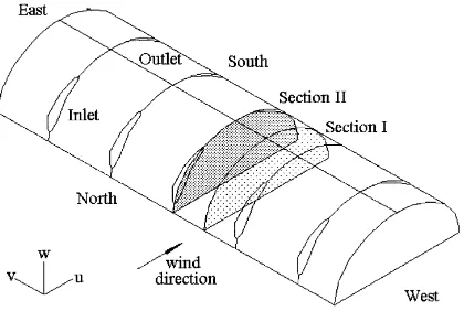
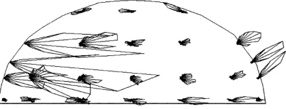
The measurements were carried out in Avignon (44◦N latitude, 5◦E longitude and 24 m altitude), in an empty 22×8 m2tunnel equipped with discontinu-ous openings obtained by separating the plastic sheets every 4 m on either side of the tunnel with pieces of wood. Schematic views of the tunnel are shown in Fig. 1. Assuming a weak influence of the gable ends
Fig. 1. Schematic plan of the experimental plastic tunnel. (u, v, ware three components of the air velocity measured by the sonic anemometer in the two sections).
and symmetric air flows along the ydirection with respect to each opening, we have explored the tun-nel’s turbulent flow characteristics in two transverse sections:
a middle section (I), situated 2 m westward from section (II) mid-way between two consecutive vent openings; and
a ‘vent’ section (II), situated in the middle of the vent openings, with a northern air inlet situated wind-ward and a southern air outlet leewind-ward.
These parallel cross-sections were in the plane of the wind direction.
In order to have a continuously evaporating soil sur-face, the tunnel was abundantly watered before, and during, experiments.
3.2. Instrumentation
Rapid fluctuations in air velocity and temperature were measured by means of two three-dimensional (3-D) sonic anemometers (omnidirectional, R3, re-search ultrasonic anemometer, Gill R&D) and air hu-midity by means of two krypton hygrometers (Camp-bell, Utah). These four instruments were used to si-multaneously sense air velocity, temperature and hu-midity fluctuations at two locations in each section. At each location, the measurement head of the krypton hygrometer was placed within 0.2 m of the sampling volume of the sonic anemometer in order to minimise the flow distortion.
With only two sampling positions possible at any one time, a difficulty arises from how to deal with changing external conditions throughout the time needed to measure the 24 different measurement posi-tions within each cross section (Fig. 2). This problem was overcome:
1. by selecting measurements for a fixed northerly external wind direction; and
by using an external reference wind speed U0
and the difference in air temperature (Ti−To) and humidity (Xi−Xo) between the centre of the green-house (subscript ‘i’) and the external air stream (subscript ‘o’) as scaling parameters.
Ti,Xi, andTo,Xo were measured 1.5 m above the
soil surface inside, and outside, the tunnel whileUo
Fig. 2. Measurement positions in the central section of the tunnel. All dimensions are in metres. (d), Air temperature, humidity and velocity measurements by 3-D sonic anemometers and krypton hygrometers (1 to 24); (×), surface temperature measurements (Ts1- Ts14); (△), reference inside air temperature and humidity measurements (Ti,Xi).
formulae is given in Appendix A. Appendix B gives relations allowing the reader to derive actual physical values from the normalised figures using the average values of the scaling parameters (U¯o, 1Tio, 1Xio)
measured during the experiment.
Three components of wind velocity, air temperature and humidity fluctuations were measured at 24 posi-tions in each section together with the thermal bound-ary conditions at 14 positions along the inside soil surface and plastic cover surface (Fig. 2). Tempera-tures were measured by means of thin thermocouples stuck on the plastic cover or soil surface. The manu-facturer’s calibration was accepted foru,v,w, air tem-perature and humidity measurements. Sampling fre-quency was 5 Hz. The time duration of each measure-ment record (for characterisation of two locations) was about 10 min.
The outside air temperature (To) and humidity (Xo),
wind speed (Uo), and direction (θ), and the inside ref-erence air temperature (Ti) and humidity (Xi) at the centre of the tunnel (Fig. 2) were measured each sec-ond and averaged over the length of each record. Ana-logue signals from the sonic anemometers and kryp-ton hygrometers were processed on-line and stored in a portable computer with eddy correlation and rapid Fourier-transform programme options. Outside, and inside, mean climatic conditions and thermal bound-ary conditions were averaged on-line and results stored in a potable data logger (Campbell CR20: Campbell, Utah).
3.3. Wind conditions
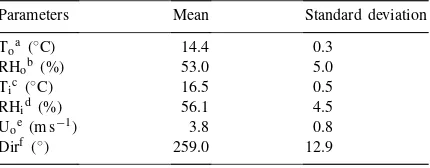
The tunnel was located at Avignon in a region char-acterised by frequent northerly winds channelled by the Rhône Valley. This wind (the Mistral) provides re-markable conditions for wind research, because of its frequency, constancy of direction (north) and persis-tence (McAneney et al., 1988). Measurements were made one day (24/10/97) during a strong Mistral with an average wind speed of 3.8 m s−1. Table 1 sum-marises prevailing weather conditions during the ex-periment and illustrates the constancy of wind direc-tion and uniformity of the main scaling parametersUo, (Ti−To), (Xi−Xo).
Table 1
Climatic boundary conditions during the experimental period Parameters Mean Standard deviation
Toa (◦C) 14.4 0.3
RHob (%) 53.0 5.0
Tic(◦C) 16.5 0.5
RHid(%) 56.1 4.5
Uoe(m s−1) 3.8 0.8
Dirf (◦) 259.0 12.9
aExterior air temperatures.
bRelative humidities of the exterior air. cInterior air temperatures.
dRelative humidities of the interior air. eExternal wind speed.
Fig. 3. Polar graph of the experimental air velocity in section I.
4. Results
4.1. Tunnel flow field
4.1.1. Polar plots
Figs. 3 and 4 show frequency distributions of air flow directions in the vertical plane (u–w) as polar plots at each position of sections I and II. The ori-gin of each plot is the measurement position and the probability densities were calculated, accumulated and plotted at 10◦ intervals from 0 to 360◦. These val-ues are plotted at the angle representing the interval mid-points and their extremities connected by a line to form the polar graph. In this way, the mean flow di-rection in theu,wplanes together with the deviations in the flow can be easily represented.
The air-flow pattern (Fig. 4) in the vent-opening sec-tion (secsec-tion II) was characterised by a very strong air stream entering through the northern opening, crossing the tunnel and escaping through the southern opening. As shown in Fig. 3, air speed was much weaker in the mid-section (section I), centred between two consec-utive openings. Here, we observed an airflow pattern characterised by two vortex, one rotating anticlock-wise and centred on the southern side of the tunnel, and a second, rotating clockwise and centred on the northern side of the tunnel.
Fig. 4. Polar graph of the experimental air velocity in section II.
4.1.2. Two-dimensional vectors
The mean vector fields are presented in Fig. 5 for section II. This shows clearly that the air stream crosses the tunnel and escapes perpendicularly through the southern vent opening. If we only consider air circulation in section II, mass conservation did not hold with the inflow exceeding the outflow. As a consequence, and contrary to our initial expectations, lateral air circulations perpendicular to the mean flow (vcomponent) were not symmetrical with respect to the middle of each vent opening.
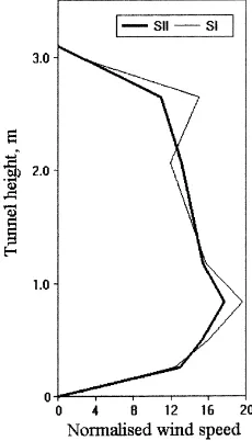
Vertical profiles of the reduced 3-D resultant air ve-locity in the middle of the tunnel (Fig. 6) were sim-ilar for both sections. Approximately the same val-ues (13<Uj*<18%) were observed between 0.25 and
2.7 m, with a peak value (Uj∗=18%) at 0.9 m and de-creasing to zero at soil and roof levels. As illustrated by the horizontal profile at 1 m height (Fig. 7), this similarity of profiles was only observed in the mid-dle section of the greenhouse. Conversely, air velocity was maximum at the air inlet (Uj∗=100%) and outlet
for sections II and I, respectively. Physical values of air-temperature (◦C) differences can be deduced by multiplying T∗ with the average difference between inside and outside (2.2◦C, see Appendix B).
Fig. 5. Normalised air velocity (expressed as a percentage of outside wind speed) distribution measured in section II.
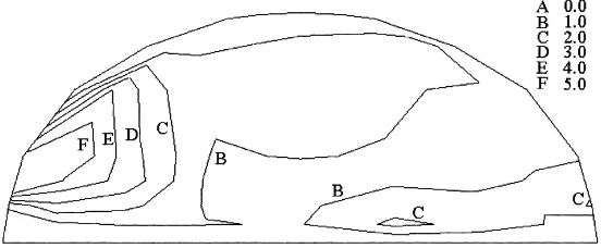
(1.5<T*<2.5). Solar absorption at soil surface also generated a vertical gradient (1.5<T*<2.5) in the first 20 cm above the soil, i.e. across the soil surface boundary layer.
4.3. Air humidity patterns
Normalised air water vapour distributions X*(j) =[{X(j,t)−Xo(t)}/{Xi(t)−Xo(t)}] are shown in Figs. 10 and 11 for sections I and II. respectively. Similar patterns were observed in both sections, with ‘dry’ regions (X*<1) situated windward in the northern and upper parts of the tunnel and the more ‘humid’ regions (1.8<X*<3) near the soil surface, where water vapour was evaporated, and concentrated in
Fig. 6. Normalised air speed (expressed as a percentage of outside wind speed) in the middle of the two sections of the tunnel.
the leeward part of the tunnel. This pattern is sig-nificantly different from that of the air temperature pattern presented above because, contrary to the heat diffusion from the cover to the inside air observed in Figs. 8 and 9, a gradient of water vapour can only be observed above the soil surface. Yet, water vapour transfer above the soil surface seemed to be more im-portant than heat diffusion, as indicated by the larger extension of the areas with 1.8<X*<3 as compared to the area with 1.8<T*<3. However, one must con-sider cautiously the humidity measurements because air humidity gradients (kg kg−1) between inside and outside were rather weak (see Appendix B).
4.4. Air turbulence characteristics
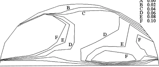
4.4.1. Turbulent kinetic energy distribution
Fig. 12 shows the map of the normalised and time averaged turbulent kinetic energy (k*(j)=(1/2) [{u′2(j,t)+v′2(j,t)+w′2(j,t)}/Uo2(t)]×100), obtained using least-squares methods for section II. Turbu-lence intensity was weak in the centre of the tunnel, and increased strongly toward the windward opening,
Fig. 8. Normalised temperature distribution (T*(j)=[{T(j,t)−To(t)}/{Ti(t)−To(t)}]) measured in section I.T(j,t),To(t)and Ti(t) are the mean temperatures (◦C) measured at timetat positionsj, outside the greenhouse and inside in the middle of the greenhouse, respectively.
Fig. 9. Normalised temperature distribution (T*(j)=[{T(j,t)−To(t)}/{Ti(t)−To(t)}]) measured in section II.T(j,t),To(t)and Ti(t) are the mean temperatures (◦C) measured at the t time at positionsj, outside the greenhouse and inside in the middle of the greenhouse, respectively.
where k*(j) was ten times larger than at the centre. The value ofk*(j) in the northern opening and in the areas situated just leeward reached 10%. It increased moderately in the leeward opening (k*(j)≈4%), when compared to the values measured in the centre of the tunnel (k*(j)<2%). However, even the stronger val-ues measured in the opening were rather low when compared to external wind conditions (k*=26%),
Fig. 10. Normalised water vapour distribution (X*(j)=[{X(j,t)−Xo(t)}/{Xi(t)−Xo(t)}]) measured in section I.X(j,t),Xo(t)and Xi(t) are the mean air humidities (kg kg−1) measured at timetat positionsj, outside the greenhouse and inside in the middle of the greenhouse, respectively.
Fig. 11. Normalised water vapour distribution (X*(j)=[{X(j,t)−Xo(t)}/{Xi(t)−Xo(t)}]) measured in section IIX(j,t),Xo(t)and Xi(t) are the mean humidities (kg kg−1) measured at timetat positionsj, outside the greenhouse and inside in the middle of the greenhouse, respectively.
Fig. 12. Normalised turbulent kinetic energy (k*(j)=(1/2)[{u′2(j,t)+v′2(j,t)+w′2(j,t)}/Uo2(t)]×100) distribution measured in section II. The values are expressed as percentages.
4.4.2. Turbulent energy dissipation rate distribution
Turbulent energy dissipation rate, ε, was calcu-lated both from spectral density analysis and from Eq. (3) and Eqs. (7)–(9). The spatial distribution of
ε obtained by least-squares analyses of sections II (Fig. 13) and I (not shown) followed the distribu-tion of turbulent kinetic energy in both the secdistribu-tions. However, while the order of magnitude of
varia-Fig. 13. Distribution of the energy dissipation rateε (m2s−2) of velocity componentuin section II.
tions in ε was approximately the same in the two sections, the rate of turbulent kinetic energy was ap-proximately five times greater in section II than in section I.
4.4.3. Integral length and time scales
Table 2
Integral length scale of the three velocity components outside (position 0) and inside (positions 1 to 24) the tunnel at sections I and II
Positions Section I SectiomII integral length integral length scale (m) scale (m)
Lint,u Lint,v Lint,w Lint,u Lint,v Lint,w 0 8.97 13.03 0.59 8.97 13.03 0.59
1 0.29 0.71 0.10 0.22 3.08 0.08
Min 0.17 0.42 0.07 0.22 0.23 0.07 Max 2.81 3.82 1.25 8.73 3.76 2.07 Mean 1.19 1.36 0.32 2.11 1.70 0.39
Fig. 14. Integral length scaleLint,u(m) distribution of velocity componentuin section II.
II. It should be noted that the mean integral length scales for theu,vandwdirections were always higher than the path distance of the sonic anemometer, and was consequently only slightly modified by our mea-surement system. The integral length scale of the u
velocity component decreases strongly from the jet inside the North vent opening, where it reaches 8.7 m -the same value as for outside. Towards -the interior of the tunnel, the turbulence is characterised by smaller eddies, with integral length scales ranging, on aver-age, between 1.8 and 0.38 m in section II and only be-tween 0.87 and 0.3 m in section I. The distribution of the integral length scale in theu-direction in section II is shown in Fig. 14.
The time required for an eddy to flow past a fixed position may be characterised by the integral time scale. Integral time scales of velocity foru, v,w di-rections were on average similar in both, sections I and II, with higher values confined close to the roof (measurement positions Nos. 14 and 18) and the soil surface (positions no. 15 and 19) in section II, and between the northern wall and the soil surface (point Nos. 22 and 23) in section I.
4.4.4. Microscale of turbulence
Fig. 15. Microscaleλ(m) distribution of velocity componentuin section II.
48 points) in section II. An equivalent dependence was earlier signalled by Heber et al. (1996) in a barn.
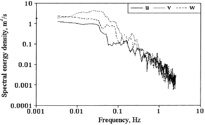
4.4.5. Energy spectra
Comparison of the energy spectra of the external wind (Fig. 16), in the vent opening at position No. 3 (Fig. 17) and that inside the tunnel at position No. 23 in section I (Fig. 18), show that the air current in the windward opening was the most turbulent, followed by the outside wind. The lowest values were found at position no. 23 between two openings. All locations had similar spectral levels at higher frequencies in the dissipation region. However, the behaviour at lower frequencies was quite divergent. In the vent opening, spectral densities at lower frequencies followed the dominance of outside conditions. Most positions with low average air speed showed very similar curves for u-, v- and w-components (see position No. 23,
Fig. 16. Spectral energy distribution of the wind at a height of 1.65 m outside the greenhouse tunnel.
section I), with a spectral decay rate correspond-ing to the high frequency spectral energies equal to about −5/3, as it is normally the case for isotropic turbulence.
5. Discussion
In experimental conditions marked by a strong external wind perpendicular to the tunnel axis and moderate inside–outside temperature and humidity differences the wind driven ventilation flux prevails substantially over the buoyancy forces (de Jong, 1990; Boulard and Draoui, 1995). In these condi-tions, the measurements demonstrated an intense air current crossing the tunnel between the windward and leeward openings, while the air along the floor and in the vertical section between two consecutive series of opening remained still. The air temperature
Fig. 18. Spectral energy distribution of the internal airflow at position 23 in section I.
and water vapour distributions were considerably influenced by these fluxes, with a high north–south gradient due to the cold and dry air penetration through the windward vent opening. The turbulence intensity notably increased from the centre of the tunnel toward the windward opening, where it was about ten times larger than in the centre of the tun-nel. These experimental data can be compared with the experimental air-speed profiles measured at crop level with the same wind conditions (wind driven ventilation in Mistral conditions) in a multispan–span greenhouse equipped with roof openings parallel to the wind direction (Wang et al., 1999 ; Haxaire et al., 1999). The average air speeds in the major volume of the tunnel were ranging between 20 and 80% of the outside wind velocity, against values between 10 and 20% only in the greenhouse equipped with roof openings. We can also observe that, contrary to the tunnel, the high air speed and turbulence intensities in the multispan greenhouse were not concerning the zones where the plants grow, but were confined near the roof openings in the upper volume of the greenhouse.
6. Concluding remarks
With the current design of vent openings, the present results demonstrated that the mean and turbulent wind conditions within a large part of the greenhouse tunnel volume were similar to those outside, particularly near the soil surface where the crops would be growing.
Plant growth would be enhanced by less heteroge-neous and turbulent conditions, so there is a require-ment for improved designs of vent opening, which would reduce the mean wind speed and the turbulence within the greenhouse tunnel. Computational fluid dy-namics (CFD) simulations could be a valuable tool for analysing and designing better greenhouse venti-lation. In this way, the size, position and shape of the vent openings can be designed so that the outdoor air mixes more smoothly at crop level with the indoor air, without forming regions with a direct penetration of outside air, or stagnant regions.
As suggested by previous CFD simulations for greenhouses (Mistriotis et al., 1997; Boulard et al., 1998), experimental validation is needed for quanti-tatively analysing the predictive accuracy of CFD in detail, and particularly the fluctuating component of the flow. The results of the present study provide both, a high-resolution database with which to validate on-going efforts with computer simulations of the mean and turbulent characteristics of the greenhouse environment and a move towards a better understand-ing of the plant environment behaviour under such conditions.
7. Notation
E spectral density (m2s−1)
L turbulent length scale (m)
R normalized autocorrelation function
f frequency (s−1)
k turbulent kinetic energy, (m2s−2)
T air temperature (◦C)
t time (s)
u horizontal air velocity, positive north to south (m s−1)
v horizontal air velocity, positive west to east (m s−1)
w vertical air velocity, positive upward (m s−1)
9. Superscripts
′ fluctuating component of quantity
in question
* reduced quantity in question
10. Symbols above letters
Physical values can be deduced from the nor-malised parameters knowing the average value of the three scaling parameters during the experiment:
¯
Boulard, T., Draoui, B., 1995. Natural ventilation of a greenhouse with continuous roof vents: measurements and analysis. J. Agric. Eng. Res. 61, 27–36.
Boulard, T., Haxaire, R., Lamrani, M.A., Roy, J.C., Jaffrin, A., 1998. Characterisation and Modelling of the air fluxes induced by natural ventilation in greenhouses. AgEng Oslo 98. International Conference in Agricultural Engineering, Oslo, 24–27 August 1998.
de Jong, T., 1990. Natural ventilation of large multi-span greenhouses. Thesis. Agricultural University, Wageningen. de Tourdonnet, S., 1998. Maˆıtrise de la qualité et de la
pollution nitrique en production de laitues sous abris plastique: diagnostique et modélisation des effets des systèmes de culture. Thèse de Doctorat de l’INA Paris–Grignon, 225 pp. Fernandez, J.E., Bailey, B.J., 1992. Measurement and prediction
of greenhouse ventilation rates. Agric. For. Meteorol. 58, 229– 245.
Haxaire, R., Boulard, T., Mermier, M., 1999. Greenhouse natural ventilation by wind forces. British–Israeli Symposium on Greenhouse Climate, Haifa, Israël, 5–10 September.
Heber, A.J., Boon, C.R., Peugh, M.W., 1996. Air patterns in an experimental livestock building. J. Agric. Eng. Res. 64, 209– 226.
Heber, A.J., Boon, C.R., 1993. Air velocity characteristics in an experimental livestock building with non-isothermal jet ventilation. ASHRAE Trans.: Symposia 99 (1), 1139–1151.
Kaimal, J.C., Finnigan, J.J., 1994. Atmospheric Boundary Layer: Oxford University Press, Oxford.
Lay, R., Bragg, G.M., 1988. Distribution of ventilation air-measurements and spectral analysis by micro-computer. Building Environm. 23 (3), 203–213.
McAneney, K.J., Baille, A., Sappe, G., 1988. Turbulence measurements during mistral winds with a 1-dimensional sonic anemometer. Bound, layer Meteorol. 42, 153–166.
Mistriotis, A., Arcidianoco, C., Picuno, P., Bot, G.P.A., Scarascia Mugnozza, G., 1997. Computational analysis of the natural ventilation in greenhouses at low wind speed. Agric. For. Meteorol. 88, 121–135.
Mohammadi, B., Pironneau, O., 1994. Analysis of thek-epsilon turbulence model. Research in Applied Mathematics, Wiley, Masson.
Pasquill, F., Smith, F.B., 1983. Atmospheric Diffusion: Wiley, New York.
![Fig. 8. Normalised temperature distribution (T*(j) = [{T(j,t) − To(t)}/{Ti(t) − To(t)}]) measured in section I](https://thumb-ap.123doks.com/thumbv2/123dok/3169609.1387560/7.612.161.437.493.603/fig-normalised-temperature-distribution-t-ti-measured-section.webp)
![Fig. 12. Normalised turbulent kinetic energy (k*(j) = (1/2)[{u′2(j,t) + v′2(j,t) + w′2(j,t)}/U2o (t)] × 100) distribution measured in section II.The values are expressed as percentages.](https://thumb-ap.123doks.com/thumbv2/123dok/3169609.1387560/8.612.163.438.230.345/normalised-turbulent-kinetic-distribution-measured-section-expressed-percentages.webp)