A COMPARISON OF SUB-PIXEL MAPPING METHODS FOR COASTAL AREAS
Qingxiang Liu*, John Trinder, Ian Turner
School of Civil and Environmental Engineering, University of New South Wales, Australia - [email protected], [email protected], [email protected]
Commission VII, WG VII/4
KEY WORDS: Sub-pixel Mapping, Coastal Areas, Soft Classification, Multispectral Images, Supervised Classification, Waterline
ABSTRACT:
This paper presents the comparisons of three soft classification methods and three sub-pixel mapping methods for the classification of coastal areas at sub-pixel level. Specifically, SPOT-7 multispectral images covering the coastal area of Perth are selected as the experiment dataset. For the soft classification, linear spectral unmixing model, supervised fully-fuzzy classification method and the support vector machine are applied to generate the fraction map. Then for the sub-pixel mapping, the sub-pixel/pixel attraction model, pixel swapping and wavelets method are compared. Besides, the influence of the correct fraction constraint is explored. Moreover, a post-processing step is implemented according to the known spatial knowledge of coastal areas. The accuracy assessment of the fraction values indicates that support vector machine generates the most accurate fraction result. For sub-pixel mapping, wavelets method outperforms the other two methods with overall classification accuracy of 91.79% and Kappa coefficient of 0.875 after the post-processing step and it also performs best for waterline extraction with mean distance of 0.71m to the reference waterline. In this experiment, the use of correct fraction constraint decreases the classification accuracy of sub-pixel mapping methods and waterline extraction. Finally, the post-processing step improves the accuracy of sub-pixel mapping methods, especially for those with correct coefficient constraint. The most significant improvement of overall accuracy is as much as 4% for the sub-pixel/pixel attraction model with correct coefficient constraint.
1. INTRODUCTION
Coastal image classification is important for the monitoring of changes of coastal features, such as shoreline position and the coverages of coastal water bodies, sandy beaches and vegetation. Compared with other data source such as aerial images and UAV-acquired images, satellite images have the advantage of large spatial coverage, which is efficient for large-scale coastal monitoring. However, the biggest disadvantage for most satellite images is the relatively low spatial resolution which limits the accuracy of estimation of coverages and positioning of boundaries. Sub-pixel mapping technique may be a solution to relieve this limitation. Generally, to realise the classification at sub-pixel level based on the original pixel-level images, two main steps are implemented: soft classification which predicts the percentage of each class inside a pixel and the pixel mapping which determines the distribution of sub-pixel labels.
Soft classification, also called sub-pixel classification, allows multiple class membership for each pixel, which is designed to overcome the mixed pixel problem (Mertens, 2008). The estimation of class proportions inside each pixel leads to the generation of multiple fraction/abundance images, which are required for the following sub-pixel mapping step. Based on multiple criteria, Heremans and Van Orshoven (2015) compared 6 commonly applied machine learning methods, i.e. Multilayer Perception, Support Vector Regression, the Least-Squares (LS)-SVM, Bagged Regression Trees, Boosted Regression Trees and Random Forests for sub-pixel land cover classification with 8-day MODIS NDVI images based on multiple criteria. They found that SVMs outperform other methods when time and training data are not considered. Other soft classification methods not belonging to machine learning include linear spectral unmixing (Settle and Drake, 1993) and fuzzy
*
Corresponding author
classification (Bastin, 1997). The soft classification step is very important in the determination of the final classification accuracy in sub-pixel level (Thornton et al., 2006, Mertens, 2008). Therefore, the comparison and selection of soft classification methods is implemented in this paper.
To date, considerable research effort has been spent on the development of sub-pixel mapping techniques. Based on the characteristics of each method, most sub-pixel mapping algorithms can be classified as two basic groups: regression based algorithms and spatial optimisation based algorithms (Atkinson, 2009). Among these algorithms, the first type includes geostatistical methods (Boucher and Kyriakidis, 2006, Boucher et al., 2008) , spatial attraction models (Mertens et al., 2006, Mertens, 2008, Liguo et al., 2011, Wang et al., 2012), Artificial Neural Networks (ANN) (Frieke, 2003, Mertens, 2008) and Wavelet Transform (Ranchin and Wald, 2000, Mertens et al., 2004, Mertens, 2008, Romberg et al., 2001). Algorithms falling into the second type include Genetic Algorithms (Mertens et al., 2003, Mertens, 2008, Michalewicz, 2013), pixel swapping (Atkinson, 2001, Atkinson, 2005, Thornton et al., 2006, Ling et al., 2008), Hopfield Neural Networks (Tatem et al., 2001a, Tatem et al., 2001b, Tatem et al., 2002, Tatem et al., 2003) and Markov Random Field (MRF) (Kasetkasem et al., 2005, Li et al., 2012, Aghighi et al., 2015). The experiments of (Mertens, 2008) indicated that the performance of each sub-pixel mapping method varies for images with different feature content. Therefore, the selection of the most proper method for coastal areas is necessary.
In this paper, Section 2 introduces the principle of selected soft classification methods and sub-pixel mapping methods. Section 3 illustrates the conduct of the experiment with SPOT-7 multispectral images and gives a comparison and discussion of results. Section 4 gives the conclusion and future work.
2. METHODOLOGIES 2.1 Selected Soft Classification Methods
In this paper, linear spectral unmixing, fully-fuzzy classification and SVM method are selected and compared for the soft classification.
2.1.1 Linear Spectral Unmixing (LSU): Linear mixture model (LMM) involves representing any kind of spectral usually applied. Firstly, the fractional abundance vector should be no less than zero. Secondly, the sum of fraction values for each pixel should be one. More details of LSU can be found from the paper by Keshava and Mustard (2002).
This method has been widely applied in the sub-pixel mapping especially for hyperspectral images with many spectral bands. The commonly used software ENVI even has the linear spectral unmixing tool to extract the endmembers. However, the main drawback of LSU is the definition of endmembers and the assumption of orthogonality (Tompkins et al., 1997, Maselli, 2001). Nevertheless, this method has been tested considering its advantages of simplicity to understand and ease for implementation.
2.1.2 Fully-fuzzy Classification (FFC): Bastin (1997) proved that fuzzy classification is more accurate than linear mixture modelling and maximum likelihood classification method for Landsat TM imagery. Further, the fully fuzzy classification method used by Zhang and Foody (2001) can relax the requirements for training pixels compared with partially-fuzzy classification, indicating that the training pixels do not need to be pure, which can be beneficial for images with relatively low spatial resolution. It outperforms the partially-fuzzy classification method as it increases the degree of overlap between pure pixels. Their method is based on the fuzzy c-means algorithm (Bezdek, 2013), while instead of the mean and covariance of the samples, the fuzzy mean vi and fuzzy membership of training sample
j classification centre
v
i will be calculated by equation (3):
weighting exponent controlling degree of fuzziness.2.1.3 Support Vector Machine (SVM): Mountrakis et al. (2011) gives a review of the increasing numbers of recent works using SVM in remote sensing area and conclude that SVM has good generalisation ability even with limited numbers of training samples. SVM can be used not only for classification but also for regression. For soft classification SVM is used for regression. The basic principle is to fit a model to predict the possibility of each pixel belonging to each class based on the training samples (Heremans and Van Orshoven, 2015). The training samples are projected to a higher-dimensional feature space by applying an appropriate kernel function. Several kernel functions can be used including the linear, polynomial, radial basis function (RBF) and sigmoid function. In this paper, the RBF is applied. In the new feature space, a linear model is then fitted with maximal margin with minimal errors. Therefore, the non-linear regression problem is solved as a linear regression function in higher-dimensional feature space (Smola and Schölkopf, 2004). There are two parameters mostly affecting the performance of the soft classification, i.e. the parameter
Three popular sub-pixel mapping methods, i.e. sub-pixel/pixel spatial attraction model, pixel swapping, ANN predicted Wavelet Transform are tested and compared in this paper. The introduction of those selected methods follows.
2.2.1 Sub-pixel/pixel Attraction Model (SAM): Spatial dependence, i.e. spatially close observations are more likely to be alike than spatially distant ones, is the basic assumption for sub-pixel mapping (Mertens et al., 2006). For spatial attraction sub-pixel mapping models, spatial dependence is expresses by the attraction of neighbouring pixel or sub-pixels. Based on the variation of attraction targets, different models such as the pixel/pixel attraction model (Liguo et al., 2011), sub-pixel/pixel model (Mertens et al., 2006) and sub-pixel/pixel attraction model (Wang et al., 2012) were developed. The main advantages of these models are the simplicity and ease of value for class cis calculated as:
,
neighbourhood models (Mertens, 2008) and the ‘surrounding’ model where all the 8-connected pixels are considered in the calculation of attraction, is selected for this paper.Figure 1. Illustration of coordinates of pixel and sub-pixel and distance calculation between them (adopted from Mertens
(2008))
After the calculation of attraction value for each class, one simple method to derive the sub-pixel mapping result is to directly label each sub-pixel with the class with largest attraction value. Alternatively, the correct fraction (CF) constraint which forces the number of sub-pixels for each class inside a pixel to be consistent with the fraction value of the soft classification result (Mertens et al., 2004) can be applied. In this paper, both SAM and SAM with CF constraint (SAM CF) will be tested.
2.2.2 Pixel Swapping (PS): PS method was firstly raised and tested on simulated imagery by Atkinson (2001) and then developed by other researchers such as Thornton et al. (2006), Luciani and Chen (2011) and Yuan-Fong et al. (2012). Firstly, the binary classification image at sub-pixel level is generated by random allocation according to the fractions of classes. Then, the attraction value
A
iof each sub-pixel from neighbouring pixels for class kis calculated by a distance-weighted function:
indicates whether the neighbouring sub-pixelj
x is labelled as class kor not (1 or 0),
ij
is the distance-dependent weighting parameter calculated as:h is the distance between sub-pixel x and its neighbour i sub-pixel proportion of each class inside each pixel is kept throughout the iteration (Thornton et al., 2006), it is a method with CF constraint.
2.2.3 ANN Predicted Wavelet Transform (ANN WT): Wavelet transform (WT) for 2D image can decompose the source image into approximation images at different lower spatial resolutions and detail coefficients forming the difference between successive approximations (Ranchin and Wald, 2000). Inversely, with the approximation fraction image and the estimated detail coefficients, the higher-resolution fraction image can be reconstructed ideally without any information loss (Mertens, 2008, Mertens et al., 2004). Mertens (2008) introduced ANN to model the wavelet coefficients considering ANN’s noise-resistance and capability of modelling. Their experimental results indicate that ANN WT method generally perform better than Genetic Algorithm and spatial attraction method. To derive the fraction image
1 j
F with higher resolution level of j1 based on the input coarse fraction
j
F in resolution level of
j
, four steps are needed as shown in Figure 2. Firstly, WT decomposition is applied to the fraction imagej
F to generate horizontal coefficient image 1
F and coefficient images 1 j H ,Vj1 and Dj1respectively. Thirdly, the modelled ANNs are used to predict the coefficient images
j with the input fraction image are generated. Finally, the fraction image
1 j
F in higher resolution level j1 is generated by WT reconstruction step.
Figure 2. Framework of ANN WT (adapted from Mertens et al. (2004))
Similar with the SAM and SAM CF methods, there are two methods, i.e. ANN predicted WT without or with the CF constraint, which will be abbreviated as ANN WT and ANN WT CF respectively in the following.
3. EXPERIMENT RESULTS AND DISCUSSION 3.1 Dataset
A set of SPOT-7 pan-sharpened sample images over Port Beach in Perth, Australia was downloaded from the website
http://www.geo-airbusds.com/en/23-sample-imagery. The images were acquired on 24 October 2014 with a spatial resolution of 1.5m and four spectral bands. A spatial subset of 1024×512 pixels is selected and the location of the studied area is shown in Figure 3. To simulate the coarse-resolution image at pixel level, each of the four spectral bands is degraded to pixel size of 6m, which means the scale factor is 4. The reference classification map in sub-pixel level is manually created using the original multispectral images. The soft classification map in pixel level is then generated by calculating the percentages of each class inside the block of every 4×4 pixels.
Figure 3. Studied area
3.2 Feature Selection and Supervised Soft Classification For the studied area of interest, five classes are pre-defined, i.e. water, sandy beach, vegetation, high-reflection objects and low-reflection objects. The high-low-reflection objects mainly include visually-bright buildings and man-made structures while the low-reflection objects are mostly roads, shadows and visually-dark roofs. 30 training pixels assumed to be ‘pure’ for each of the pre-defined class are manually selected for LSU method; considering the large coverage of water body, 50 training pixels are selected. The training pixels are marked as crosses in different colours for different classes shown as Figure 4(a).
Endmembers are extracted by simply averaging the training sample vectors belonging to the same class.
For SVM, the same set of training pixels is selected. Apart from the intrinsic attributes of the original images, i.e. the pixel values corresponding to multispectral bands, other attributes including Normalised Difference Vegetation Index (NDVI) and Difference Water Index (NDWI) (Gao, 1996) are also selected and added to the input features vectors to improve the accuracy of the soft classification. Moreover, the position of the pixel, i.e. the row and column are selected as well considering the spatial distribution of different objects. All those features are scaled to the range of [-1, 1] to avoid the features with much larger numeric values dominating other features. The open source package LIBSVM developed by Chang and Lin (2011)
distributed on the website
https://www.csie.ntu.edu.tw/~cjlin/libsvmtools/ were downloaded and utilised for the processing. To find the optimal combination of parameter
and c , the parameter optimisation tool applying cross validation (CV) to the training samples is used. According to the optimisation result, the optimal parameters are 4.0 and 0.25 respectively.To be consistent with SVM and LSU method, the same number of training pixels with the SVM method is selected for FFC. However, some of those training pixels are changed to mixed pixels as shown in Figure 4(b) with fraction values all above 0.9. The optimal value 2.3 of weighting exponent parameter m
is derived by initial analysis to minimise the mean root mean square error (RMSE) of the five classes. Table 1 gives the accuracy of the soft classification results including the RMSE and correlation coefficient (CC) for each class.
(a) (b)
Figure 4. (a) Training pixels for LSU and SVM. (b) Training pixels for FFC.
water Sandy beach
vegetat ion
High-reflection
objects
Low-reflection
objects
RMSE LSU 0.165 0.128 0.171 0.122 0.298
FFC 0.052 0.174 0.205 0.373 0.445
SVM 0.048 0.107 0.125 0.099 0.173
CC LSU 0.953 0.874 0.783 0.769 0.812
FFC 0.995 0.782 0.638 0.437 0.495
SVM 0.997 0.917 0.835 0.858 0.922
Table 1. Accuracy assessment of soft classification methods
It can be seen that the SVM performs best no matter whether judged based on RMSE or correlation coefficient. Specifically, it generates the most accurate result for the classification of water body with RMSE of 0.048 and correlation coefficient of 0.997. LSU is generally better than FFC except for the classification of water body. This can be explained by the intra-class variability between still water body and the nearshore water body with highly-reflective foams and waves. The selection of training pixels within this area can significantly affect the resultant spectrum of endmember.
The FFC method is almost as accurate as SVM for the classification of water body with RMSE of 0.052 and correlation coefficient of 0.995, while for other classes it generates the poorest result. Although the FFC method does not generate as good result as SVM, it has the advantage of the relaxation of training pixels. This can be very crucial when it is difficult to choose pure pixels or even when there are no pure pixels for some classes, which does not satisfy the basic assumption of many algorithms. Since the soft classification result directly determines the final results, the SVM method is used in the following.
3.3 Sub-pixel Mapping
In order to compare the sub-pixel mapping techniques with pixel-level classification, the hard classification result of SVM at pixel level is resized to the same dimension as the sub-pixel result, which is abbreviated as HC for convenience. Besides, to improve the performance of PS method, the ANN WT CF result is used as initial input instead of random distribution. The results of the selected sub-pixel mapping methods are shown as Figure 5. It can be seen that for all the methods, some parts of the wet sandy beach are misclassified as low-reflection objects. Although for those methods without CF constraint many small objects are lost, especially for the SAM method; methods with CF constraint seem to be less accurate since they generate many scattered pixels or patches.
(a) (b) (c)
(d) (e) (f)
(g)
Figure 5. Sub-pixel mapping results where blue, yellow, white and grey pixels represent water body, sandy beach, high-reflection objects and low-high-reflection objects. (a) Reference map. (b) HC. (c) ANN WT. (d) ANN WT CF. (e) SAM. (f) SAM CF. (g) PS.
The Cohen's Kappa coefficient and overall accuracy (OA) for those methods are presented in Table 2. Firstly, ANN WT generates the most accurate result with OA and Kappa coefficient of 91.3% and 0.867 respectively, followed by SAM method with OA and Kappa coefficient of 91.21% and 0.865. However, even for the most accurate two methods, i.e. ANN WT and SAM, the accuracy does not improve much compared with the hard classification result using SVM. The increase of OA for them is only 0.21% and 0.12% respectively. Secondly, as consistent with visual judgment, the methods without CF constraint generate more accurate results than those with CF and the HC. By applying CF constraint, the accuracy decreases considerably, which is even worse than HC. Taking the most accurate ANN WT as an example, after applying CF, the accuracy reduces to the lowest. Thirdly, among the three methods with CF constraint, PS is the most accurate one with OA and Kappa coefficient of 88.79 and 0.831 respectively.
OA (%) Kappa
HC 91.09 0.864
ANN WT 91.30 0.867
ANN WT CF 87.41 0.809
SAM 91.21 0.865
SAM CF 87.44 0.809
PS 88.79 0.831
Table 2. Accuracy assessment of sub-pixel mapping methods
3.4 Post-processing
To improve the final results, a post-processing step incorporating known geographic knowledge is implemented. Firstly, it is believed that the water body should be only one connected region and isolated water body areas are reclassified. While this might not hold for some special areas, it can reduce the misclassification for most cases of coastal areas.
Secondly, very small patches are regarded as misclassified. Verhoeye and De Wulf (2002) used a smoothing filter to reduce the isolated sub-pixels in their sub-pixel mapping results, which is a reverse step of sub-pixel mapping (Mertens, 2008), while in this paper, filtering is avoided. Instead, they are re-labelled according to the available information. For ANN WT and ANN WT CF, each of these sub-pixels is reclassified to the class with second largest fraction value. Similarly for SAM and SAM CF, they are reclassified to the class with the second largest attraction value. For PS, since no information in sub-pixel level is available, each sub-pixel is reclassified to the class with largest number of sub-pixels shown in its neighbourhood window.
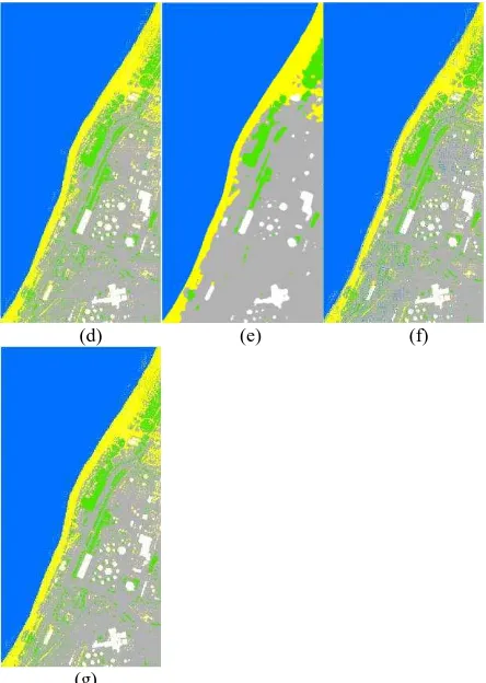
Thirdly, the areas classified as high-reflection or low-reflection objects between sandy beach and the water body or inside the water body are assumed to be misclassified and are re-labelled as water or sandy beach. This misclassification might be caused by foam and waves which are highly reflective and more similar to high-reflection objects rather than water body or by wet sand which is dark and more similar to low-reflection objects. This phenomenon is hard to avoid even with some training points in those ambiguous areas. The sub-pixel mapping results after post-processing are shown in Figure 6.
(a) (b) (c)
(d) (e) (f)
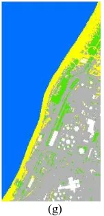
(g)
Figure 6. Post-processed sub-pixel mapping results. (a) The reference map. (b) HC. (c) ANN WT. (d) ANN WT CF. (e) SAM. (f) SAM CF. (g) PS.
The accuracy and its improvement compared with the results without post-processing are shown as Table 3.
OA (%)
Improvement of OA (%)
Kappa Improvement of Kappa
HC 91.51 0.43 0.870 0.007
ANN WT
91.79 0.48 0.875 0.008
ANN WT CF
91.36 3.95 0.868 0.059
SAM 91.29 0.08 0.866 0.001
SAM CF 91.44 4.00 0.869 0.060
PS 91.27 2.48 0.867 0.036
Table 3. Accuracy of post-processed results
After post-processing, the ANN WT is still the most accurate, which is slightly better than HC. The accuracy of HC is also improved and is more accurate than other methods except for ANN WT. The methods with CF constraint are improved considerably and the improvement of SAM CF is the most significant with 4.00% and 0.06 of OA and Kappa coefficient respectively, which is even more accurate than SAM. SAM CF and ANN WT CF are comparable with HC result after post-processing, which indicates that the methods with CF constraint can be potentially improved with proper post-processing. Since the waterline is a very important feature of coastal areas, the waterlines are extracted from the post-processed classification maps. The distance of each pixel in the extracted shoreline to the reference waterline is recorded. The mean value and RMSE of the distances for each extracted waterline are shown in Table 4.
HC ANN
WT
ANN WT
CF
SAM SAM
CF PS
Mean distance (pixels)
0.74 0.47 1.06 0.80 1.11 1.07
RMSE (pixels)
0.98 0.67 1.42 1.03 1.50 1.41
Maximum distance (pixels)
3.16 2.68 5.00 2.68 4.92 4.92
Table 4. Waterline accuracy assessment
From Table 5, we can find that ANN WT not only performs best at classification, but also generates the most accurate waterline with mean distance of 0.47 pixels, RMSE of 0.67 pixels and maximum distance of 2.68 pixels. Other methods are still not as good as HC, which is consistent with the classification accuracy assessment. However, all the methods with CF constraint generate poorer results than those without CF constraint, which indicates the CF constraint is not beneficial for the mapping accuracy of boundaries between gradually changed classes such as the waterline along sandy beaches. The errors inherited from the soft map force the sub-pixels to be assigned to classes and further result in many small patches around the boundary position. Therefore, it is expected that CF is more appropriate for areas with many small objects. Besides, the accurate soft classification map is crucial.
In the future, real coarse-resolution images instead of simulated images will be used for the objective assessment of sub-pixel mapping techniques. Besides, MRF based methodologies such as the fully spatially adaptive sub-pixel mapping method (Aghighi et al., 2014) will be compared with the ANN WT method. Moreover, the soft classification accuracy is expected to be improved by incorporating other information such as the texture information. Finally, more factors should be considered in the future if we want to assess one sub-pixel mapping method objectively and comprehensively. For example, Ling et al. (2008) found that pixel swapping method generated very different results with different scale factors, while for this paper, only the scale factor of 4 is tested.
4. CONCLUSIONS
In this work, a set of SPOT-7 multispectral images is used to test the performance of soft classification methods and sub-pixel mapping methods for the classification of coastal areas in sub-pixel level. Firstly, for the soft classification, LSU model, FFC and the SVM methods are used to generate the fraction map. The RMSE and correlation coefficient of the fraction values both indicate that SVM is the most accurate among the three methods. Then by using the soft map generated by SVM, SAM, SAM CF, ANN WT, ANN WT CF and PS methods are tested for their performance of sub-pixel mapping. A post-processing step according to the known spatial knowledge of coastal areas is then implemented to improve the results. By the accuracy assessment of the classification and waterline extraction results, ANN WT is found to be the most accurate sub-pixel mapping method compared with the other five methods. Specifically, the overall classification accuracy of ANN WT is 91.79% and Kappa coefficient of 0.875 after the post-processing step; the mean distance of the extracted waterline to the reference waterline is 0.47 pixels, i.e. 0.71m. Besides, it is found that the CF constraint decreases the classification accuracy of sub-pixel mapping methods and waterline extraction for the studied coastal area. Finally, the post-processing can be very important for some methods especially for those with CF constraint with the most significant improvement of overall accuracy is as much as 4% for the SAM CF method.
REFERENCES
AGHIGHI, H., TRINDER, J., LIM, S. & TARABALKA, Y. 2014. Improved adaptive Markov random field based
super-resolution mapping for mangrove tree identification. ISPRS Ann. Photogramm. Remote Sens. Spatial Inf. Sci., II-8, 61-68.
AGHIGHI, H., TRINDER, J., LIM, S. & TARABALKA, Y. 2015. Fully spatially adaptive smoothing parameter estimation for Markov random field super-resolution mapping of remotely sensed images. International Journal of Remote Sensing, 36, 2851-2879.
ATKINSON, P. M. Super-resolution target mapping from softclassified remotely sensed imagery. Proc. of the 6th International Conference on Geocomputation, Brisbane, University of Queensland, 2001.
ATKINSON, P. M. 2005. Sub-pixel Target Mapping from Soft-classified, Remotely Sensed Imagery. Photogrammetric Engineering & Remote Sensing, 71, 839-846.
ATKINSON, P. M. 2009. Issues of uncertainty in super-resolution mapping and their implications for the design of an inter-comparison study. International Journal of Remote Sensing, 30, 5293-5308.
BASTIN, L. 1997. Comparison of fuzzy c-means classification, linear mixture modelling and MLC probabilities as tools for unmixing coarse pixels. International Journal of Remote Sensing, 18, 3629-3648.
BEZDEK, J. C. 2013. Pattern recognition with fuzzy objective function algorithms, Springer Science & Business Media.
BOUCHER, A. & KYRIAKIDIS, P. C. 2006. Super-resolution land cover mapping with indicator geostatistics. Remote Sensing of Environment, 104, 264-282. BOUCHER, A., KYRIAKIDIS, P. C. &
CRONKITE-RATCLIFF, C. 2008. Geostatistical Solutions for Super-Resolution Land Cover Mapping. Geoscience and Remote Sensing, IEEE Transactions on, 46, 272-283.
CHANG, C.-C. & LIN, C.-J. 2011. LIBSVM: A library for support vector machines. ACM Transactions on Intelligent Systems and Technology (TIST), 2, 27. FRIEKE, V. 2003. Design and application of artificial neural
networks for digital image classification of tropical savanna vegetation.
GAO, B.-C. 1996. NDWI—A normalized difference water index for remote sensing of vegetation liquid water from space. Remote Sensing of Environment, 58, 257-266.
HEREMANS, S. & VAN ORSHOVEN, J. 2015. Machine learning methods for sub-pixel land-cover classification in the spatially heterogeneous region of Flanders (Belgium): a multi-criteria comparison. International Journal of Remote Sensing, 36, 2934-2962.
KASETKASEM, T., ARORA, M. K. & VARSHNEY, P. K. 2005. Super-resolution land cover mapping using a Markov random field based approach. Remote Sensing of Environment, 96, 302-314.
KESHAVA, N. & MUSTARD, J. F. 2002. Spectral unmixing. Signal Processing Magazine, IEEE, 19, 44-57. LI, X., DU, Y. & LING, F. 2012. Spatially adaptive smoothing
parameter selection for Markov random field based sub-pixel mapping of remotely sensed images. International Journal of Remote Sensing, 33, 7886-7901.
LIGUO, W., QUNMING, W. & DANFENG, L. Sub-pixel mapping based on sub-pixel to sub-pixel spatial attraction model. Geoscience and Remote Sensing Symposium (IGARSS), 2011 IEEE International, 24-29 July 2011 2011. 593-596.
LING, F., XIAO, F., DU, Y., XUE, H. P. & REN, X. Y. 2008. Waterline mapping at the subpixel scale from remote sensing imagery with high ‐resolution digital elevation models. International Journal of Remote Sensing, 29, 1809-1815.
LUCIANI, P. & CHEN, D. 2011. The impact of image and class structure upon sub-pixel mapping accuracy using the pixel-swapping algorithm. Annals of GIS, 17, 31-42.
MASELLI, F. 2001. Definition of Spatially Variable Spectral Endmembers by Locally Calibrated Multivariate Regression Analyses. Remote Sensing of Environment, 75, 29-38.
MERTENS, K. 2008. Towards sub-pixel mapping: design and comparison of techniques. Proefschrift Universiteit Gent, s.n.].
MERTENS, K. C., DE BAETS, B., VERBEKE, L. P. C. & DE WULF, R. R. 2006. A sub‐pixel mapping algorithm based on sub‐pixel/pixel spatial attraction models. International Journal of Remote Sensing, 27, 3293-3310.
MERTENS, K. C., VERBEKE, L. P. C., DUCHEYNE, E. I. & DE WULF, R. R. 2003. Using genetic algorithms in sub-pixel mapping. International Journal of Remote Sensing, 24, 4241-4247.
MERTENS, K. C., VERBEKE, L. P. C., WESTRA, T. & DE WULF, R. R. 2004. Sub-pixel mapping and sub-pixel sharpening using neural network predicted wavelet coefficients. Remote Sensing of Environment, 91, 225-236.
MICHALEWICZ, Z. 2013. Genetic algorithms+ data structures= evolution programs, Springer Science & Business Media.
MOUNTRAKIS, G., IM, J. & OGOLE, C. 2011. Support vector machines in remote sensing: A review. ISPRS Journal of Photogrammetry and Remote Sensing, 66, 247-259. RANCHIN, T. & WALD, L. 2000. Fusion of high spatial and spectral resolution images: the ARSIS concept and its implementation. Photogrammetric Engineering and Remote Sensing, 66, 49-61.
ROMBERG, J. K., HYEOKHO, C. & BARANIUK, R. G. 2001. Bayesian tree-structured image modeling using wavelet-domain hidden Markov models. Image Processing, IEEE Transactions on, 10, 1056-1068. SETTLE, J. J. & DRAKE, N. A. 1993. Linear mixing and the
estimation of ground cover proportions. International Journal of Remote Sensing, 14, 1159-1177.
SMOLA, A. J. & SCHÖLKOPF, B. 2004. A tutorial on support vector regression. Statistics and computing, 14, 199-222.
TATEM, A., LEWIS, H., ATKINSON, P. & NIXON, M. Super-resolution mapping of urban scenes from IKONOS imagery using a Hopfield neural network. Geoscience and Remote Sensing Symposium, 2001. IGARSS'01. IEEE 2001 International, 2001a. IEEE, 3203-3205.
TATEM, A. J., LEWIS, H. G., ATKINSON, P. M. & NIXON, M. S. 2001b. Super-resolution target identification from remotely sensed images using a Hopfield neural network. Geoscience and Remote Sensing, IEEE Transactions on, 39, 781-796.
TATEM, A. J., LEWIS, H. G., ATKINSON, P. M. & NIXON, M. S. 2002. Super-resolution land cover pattern prediction using a Hopfield neural network. Remote Sensing of Environment, 79, 1-14.
TATEM, A. J., LEWIS, H. G., ATKINSON, P. M. & NIXON, M. S. 2003. Increasing the spatial resolution of agricultural land cover maps using a Hopfield neural network. International Journal of Geographical Information Science, 17, 647-672.
THORNTON, M. W., ATKINSON, P. M. & HOLLAND, D. A. 2006. Sub‐pixel mapping of rural land cover objects from fine spatial resolution satellite sensor imagery using super ‐ resolution pixel ‐ swapping. International Journal of Remote Sensing, 27, 473-491.
TOMPKINS, S., MUSTARD, J. F., PIETERS, C. M. & FORSYTH, D. W. 1997. Optimization of endmembers for spectral mixture analysis. Remote Sensing of Environment, 59, 472-489.
VERHOEYE, J. & DE WULF, R. 2002. Land cover mapping at sub-pixel scales using linear optimization techniques. Remote Sensing of Environment, 79, 96-104.
WANG, F. 1990. Improving remote sensing image analysis through fuzzy information representation. Photogrammetric engineering and remote sensing (USA).
WANG, Q., WANG, L. & LIU, D. 2012. Integration of spatial attractions between and within pixels for sub-pixel mapping. Systems Engineering and Electronics, Journal of, 23, 293-303.
YUAN-FONG, S., FOODY, G. M., MUAD, A. M. & KE-SHENG, C. 2012. Combining Pixel Swapping and Contouring Methods to Enhance Super-Resolution Mapping. Selected Topics in Applied Earth Observations and Remote Sensing, IEEE Journal of, 5, 1428-1437.
ZHANG, J. & FOODY, G. M. 2001. Fully-fuzzy supervised classification of sub-urban land cover from remotely sensed imagery: Statistical and artificial neural network approaches. International Journal of Remote Sensing, 22, 615-628.