Subsurface equatorial zonal current in the eastern Indian Ocean
Iskhaq Iskandar,1,2 Yukio Masumoto,1,3 and Keisuke Mizuno1
Received 9 November 2008; revised 9 April 2009; accepted 16 April 2009; published 9 June 2009.
[1] Variations of subsurface zonal current in the eastern equatorial Indian Ocean are
investigated by examining 6-year data (December 2000–November 2006) from acoustic Doppler current profiler (ADCP) mooring at 0°S, 90°E. The analysis indicates the presence of an eastward equatorial subsurface current between 90 and 170 m depths during both boreal winter and summer. During boreal winter, the generation of eastward pressure gradient, which drives an eastward flow in the thermocline, is caused primarily by upwelling equatorial Kelvin waves excited by prevailing easterly winds. On the other hand, the downwelling Rossby waves generated by the reflection of the spring downwelling Kelvin waves in the eastern boundary, as well as the upwelling equatorial Kelvin waves triggered by easterlies, create an oceanic state that favors the generation of the eastward pressure gradient during boreal summer. The subsurface current reveals a distinct seasonal asymmetry. The maximum eastward speed of 63 cm s1is observed in April, and secondary maximum of 49 cm s1is seen in October. The zonal transport per unit width within depth of the subsurface current exhibits similar variations: reaching maximum eastward transport of 35 m2s1in April and secondary maximum of 29 m2s1 in October. Moreover, the subsurface current during boreal summer undergoes significant interannual variations; it was absent in 2003, but it was anomalously strong during 2006.
Citation: Iskandar, I., Y. Masumoto, and K. Mizuno (2009), Subsurface equatorial zonal current in the eastern Indian Ocean,
J. Geophys. Res.,114, C06005, doi:10.1029/2008JC005188.
1. Introduction
[2] It is generally believed that the equatorial undercurrent (EUC) is mainly forced by eastward zonal pressure gradient along the equator generated by prevailing easterlies [Cane, 1980;Philander and Pacanowski, 1980;McCreary, 1981]. Over the Pacific and Atlantic Oceans, the prevailing easterly trade winds forced a quasi-permanent eastward pressure gradient leading to the presence of the EUC throughout the year [Yu and McPhaden, 1999;Stalcup and Metcalf, 1966]. On the other hand, a distinct seasonal cycle associated with the Asian-Australian monsoon dominates the atmospheric circulation over the Indian Ocean. Thus different oceanic structures are expected to occur in the Indian Ocean in response to such wind-forcing, which is quite different from the conditions in the other basins.
[3] Early measurements along the equatorial Indian Ocean between 53°E and 92°E were conducted during the southwesterly monsoon of 1962 and the northeasterly monsoon of 1963 [Knauss and Taft, 1964]. Their data provide evidence that a somewhat weaker and more variable undercurrent than that found in the Pacific was present in
the Indian Ocean, and more clearly observed in the eastern part of the basin. Moreover, time series of equatorial currents measurements (January 1973 – September 1974) at Gan (0.5°S, 73°E) revealed a similar picture [Knox, 1976]. However, the EUC was only present during the end of northeasterly monsoon of 1973, while it was absent during 1974. Yet, in a more recent study, current measurements across 80°E between 1°S and 5°N from July 1993 to September 1994 showed the existence of the EUC during the northeasterly and southwesterly monsoon of 1994 [Reppin et al., 1999].
[4] The conditions for the EUC occurrence in the Indian Ocean are still under debate [Knox, 1976; Cane, 1980;
Reppin et al., 1999]. Knox [1976] attributed the absence of the EUC in 1974 to the weak easterly winds observed in the early months of 1974. Similarly, Reppin et al. [1999] suggested that the occurrences of the EUC during 1994 are forced by easterlies in the same year, driving an eastward zonal pressure gradient that forces the undercurrent. On the other hand, Cane [1980] proposed that the interannual variation in the EUC is determined by the winds during the late months of the previous year. The presence of EUC during the spring of 1973 is preceded by weak eastward winds in the last quarter of the preceding year, while there were strong eastward winds from early fall to early winter of 1973 leading to the absence of the EUC in spring of 1974. [5] Because of the strong time dependence of the EUC and lack of observation in the Indian Ocean, dynamical understanding of the subsurface zonal current in this peculiar ocean basin is still limited, in particular, in the JOURNAL OF GEOPHYSICAL RESEARCH, VOL. 114, C06005, doi:10.1029/2008JC005188, 2009
Click Here for Full Article
1Institute of Observational Research for Global Change, Japan Agency for Marine-Earth Science and Technology, Yokosuka, Japan.
2On leave from Jurusan Fisika, FMIPA, Universitas Sriwijaya, Palembang, Sumatra Selatan, Indonesia.
3
Also at Department of Earth and Planetary Science, Graduate School of Science, University of Tokyo, Tokyo, Japan.
eastern basin where the EUC structure is more apparently developed [Knauss and Taft, 1964]. In this study, we present the evidence of the subsurface zonal current in the eastern Indian Ocean using 6-year data from acoustic Doppler current profiler (ADCP) mooring at 0°S, 90°E.
[6] The remainder of this paper is organized as follows. Detailed description of the data sets used in this study is presented in section 2. Section 3 then shows temporal variations of the observed zonal currents. Characteristics of the observed subsurface zonal currents and mechanism responsible for the generation of the subsurface zonal current are presented in sections 4 and 5, respectively. In section 6, we discuss the interannual variations of the subsurface zonal current, especially during boreal summer. The last section is reserved for summary and discussion.
2. Data
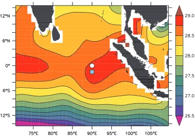
[7] An upward-looking subsurface ADCP mooring has been deployed at 90°E right on the equator since 14 November 2000 (Figure 1) [Masumoto et al., 2005]. This observed data now became the longest currents data avail-able for the equatorial Indian Ocean. The ADCP measures currents from the sea surface down to 400 m depth, with vertical interval of 10 m. However, to avoid contamination of signals reflected at the surface as well as the limited data coverage in the deeper level, only the data between the depths of 40 m and 300 m are used in this study. The daily climatology of the zonal current is calculated from time series over a period of December 2000 – November 2006.
[8] Since October 2004, two ATLAS buoys have been deployed along the equator at 80.5°E and 90°E as part of
Research Moored Array for African-Asian-Australian
Monsoon Analysis and Prediction (RAMA) program
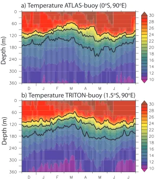
[McPhaden et al., 2009]. The buoy measures vector winds, air temperature, relative humidity, sea surface temperature (SST), and subsurface temperature from 10 m down to 500 m depth. However, data return for temperature from ATLAS buoy at 90°E is only about 46% (8 months) during October 2004 – December 2006, which hindered us from precisely analyzing the data. In order to examine variations in subsurface temperature and salinity associated with the occurrence of the EUC, data from TRITON buoy moored at 1.5°S, 90°E are used (Figure 1) [Kuroda, 2002;Hase et al., 2008]. The data were collected from 26 October 2001 using Sea-Bird Electronics model SBE37 in the upper 750 m. The gaps are filled in by applying vertical and/or temporal interpolation of Akima spline method [Akima, 1970]. The climatology of temperature and salinity is computed over a period of January 2002 – December 2006. To examine whether the mooring site is suitable for the analysis of the EUC, we compare the temperature data from TRITON buoy with that from ATLAS buoy at 0°S, 90°E for period of December 2004 to July 2005 (Figure 2). The time-depth evolution of temperature at two mooring locations agrees very well, in particular at the seasonal timescale that we are focusing on in the present study. Correlation coefficients of isotherms at each depth are exceeding 0.65 (significant at the 95% confidence level from a two-tailed Studentt-test). The doming of thermocline observed by ATLAS buoy during February – March is also appear in TRITON buoy data. However, the thermocline at ATLAS buoy is slightly tighter during January than that at TRITON buoy. In addition, the deepening of the thermocline during May is more prominent at ATLAS buoy. Despite the small differences in short-term variations between the two locations, we expect that the TRITON buoy is useful to describe the subsurface temper-Figure 1. Positions of the ADCP mooring (circle) and TRITON buoy (square) superimposed on the
annual mean sea surface temperature (°C) from World Ocean Atlas 1998.
ature variations associated with the occurrences of the subsurface zonal current.
[9] To explore dynamical balance of the subsurface zonal current, we also used monthly gridded temperature and salinity data obtained by the Argo floats [Hosoda et al., 2006]. The available Argo data have been gridded into two-dimensional map using an optimal interpolation (OI) method [Mizuno, 1995; White, 1995]. The resulting data cover the global ocean with horizontal resolution of 1°and there are 25 levels in vertical from 10 to 2000 dbar. The data are available from January 2001 to present.
[10] In addition, merged sea surface height (SSH) from AVISO and the daily winds from the SeaWinds scatterometer on the QuikSCAT for a period of January 2001 to December 2006 are also used. Mean climatologies of pressure, SSH and winds were calculated from time series over a period of January 2001 – December 2006. Note that, anomaly fields
for all variables were constructed on the basis of the devia-tions from their mean climatologies. Table 1 presents a summary of data used in this study.
3. Temporal Variations
[11] Figure 3 shows time series of the observed zonal currents at 0°S, 90°E, to which a 5-day running mean has been applied to remove high-frequency variations. One of the most prominent features of the observed zonal current in the upper layer shallower than about 90 m is the semiannual Wyrtki jets, with maximum values of more than 70 cm s1. In addition to this semiannual cycle, the time series also show a pronounced oscillation at period of about one month.
Masumoto et al. [2005] have suggested that this shorter timescale variation is a result of wind-forced variability associated with intraseasonal oscillations in the atmosphere. Figure 2. Time-depth evolution of temperatures at (a) ATLAS buoy and (b) TRITON buoy from
December 2004 to July 2005. The 15°C, 20°C, and 25°C isotherms are highlighted.
Table 1. Summary of Data Used in the Present Study
Data Interval Record Length Calculation of Climatology
Moreover, recent modeling study demonstrated that the intraseasonal variations in the upper layer zonal currents during boreal summer are forced by intraseasonal westerly burst of summer monsoon [Senan et al., 2003].
[12] In the subsurface layer below about 90 m, the observed zonal currents also indicate strong variations with longer timescale. Eastward subsurface current prevails during January – April and July – September in general, and changes its direction during other periods. The eastward undercurrent during January – April seems to be a robust feature of the subsurface structure at this location.
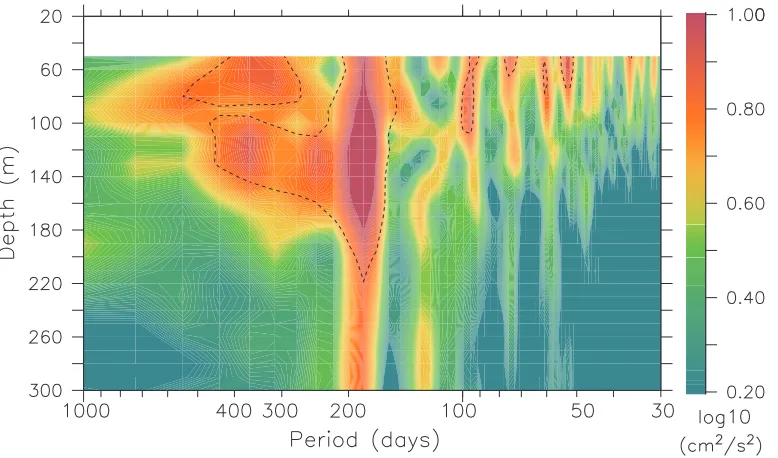
[13] Power spectra of the observed zonal current at 0°S, 90°E is shown in Figure 4. The observed zonal currents show a maximum variance in excess of 10 cm2s2at period of 180 days, which is obviously observed at depth between 70 – 180 m. While the surface layer shallower than about 90 m indicates variances at intraseasonal timescale (30 – 100 days), the subsurface layer only shows small variances at these periods. The secondary peak of the subsurface layer is apparent at annual timescale (360 days).
[14] A few existing observational studies in the western and central equatorial Indian Ocean have reported the presence of eastward subsurface current in the Indian Ocean during southwesterly monsoon [Bruce, 1973;Reppin et al., 1999] as well as during northeasterly monsoon [Knauss and Taft, 1964; Knox, 1976; Reppin et al., 1999]. Since the subsurface zonal current seems to be driven by a different mechanism from that for the surface layer and we focus here on the eastward current, we call it as EUC throughout this paper. The EUC is defined as an eastward undercurrent in and around the thermocline in the depth ranges from 90 to 170 m that lies beneath the surface westward or even weak eastward currents. This particular depth range is selected to isolate the effect of surface eastward jets known as the Wyrtki jets.
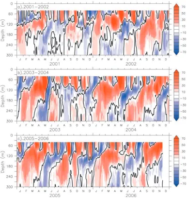
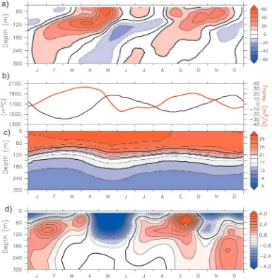
4. Characteristic of Subsurface Zonal Currents [15] Figure 5a shows the daily climatology of the zonal velocity (u) component at 0°S, 90°E. It is shown that the Figure 3. Time-depth section of the observed zonal currents (cm s1) at 0°S, 90°E from 1 January
2001 – 3 December 2006. A 5-day running mean has been applied to remove higher-frequency variations. The eastward (westward) currents are shaded red (blue), and the zero contours are highlighted.
EUC exhibits pronounced semiannual variations and upward phase propagation. An examination on the semiannual variation indicates that the amplitude has a significant peak of 28 cm s1 at depth of 120 m. The maximum eastward speed of 63 cm s1 is observed in April and secondary maximum of 49 cm s1 is seen in October. The mass transport per unit width, obtained by integrating the zonal current over the depths where the EUC is defined, also shows semiannual variations (Figure 5b). The maximum transport in April is 35 m2s1, while it is just 29 m2s1in October.
[16] Accompanying this semiannual variation is change in the vertically integrated temperature which is proportional to the heat content. Note that the integration is calculated over a similar depth where the EUC is defined. The mini-mum heat content is observed during February – March and August – September and coincides with the developing phase of the EUC (Figure 5b). This is also confirmed with doming structures of isotherms appeared twice a year (Figure 5c). The semiannual EUC, moreover, is co-occurred with a distinct seasonal variation of subsurface eastward pressure gradient (Figure 5d). We will return to this point later in the following section.
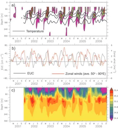
[17] The time-depth variations of the zonal velocity component at 0°S, 90°E are shown in Figure 6a along with the isothermal variability at 1.5°S, 90°E. The zonal velocity component is representative of the core of the EUC, where only values greater than 24 cm s1are shown. The EUC is constantly observed at the end of boreal winter (February – April). A similar eastward subsurface current but with weaker amplitude is also observed during boreal summer (July – September). The core of these eastward undercurrents is located within the thermocline (Table 2) and its position varies with the thermocline. An exception to the boreal summer EUC occurs in 2003.
[18] The onset of the EUC in both seasons coincides with the shoaling of thermocline, where boreal summer shoaling
indicates strong interannual variations. We note that the shoaling of thermocline during July 2003 was suddenly depressed by the presence of energetic instraseasonal surface eastward currents forced by instraseasonal winds (Figure 6b). On the other hand, the thermocline variations during the latter half of 2006 underwent a dramatic change compared to the normal condition. The shoaling of thermocline started in June, earlier than usual and it still shoaling until the mooring was recovered on December 2006. Moreover, the spreading of thermocline is more clearly observed during this period and the 25°C isotherm reached its minimum depth of about 70 m during October – December.
[19] The observed salinity fields also indicate semiannual variations (Figure 6c). There is an increase of salinity after the EUC is established. Previous studies have shown that high-salinity water seen in the eastern equatorial Indian Ocean originated from the western region [Han and McCreary, 2001;Hase et al., 2008].
[20] In order to determine the forcing of the EUC, squared coherency was calculated between the zonal winds along the equatorial Indian Ocean and the EUC (Figure 7). It is shown that on the semiannual timescale, the EUC is highly correlated with the winds from 45°E to about 85°E. The phase difference between the EUC and the zonal winds indicated that the EUC lags the winds at 60°E by about 35 days (Figure 7b). This time-lag correlation indicates an eastward propagation with phase speed about 1.1 m s1. This estimated phase speed falls between the theoretical values of the second and third baroclinic modes. Similar result was obtained byHase et al.[2008] for the semiannual variations of temperature at 1.5°S, 90°E.
5. Role of Equatorial Waves in the Evolution of Eastward Pressure Gradient
[21] It was suggested that the EUC are primarily driven by eastward pressure gradient generated by the easterly Figure 4. Power spectra (cm2s2) of the observed zonal currents at 0°S, 90°E. The values are shown in
natural logarithm (log10). Dashed contours are the 95% significance level.
winds [Cane, 1980; Philander and Pacanowski, 1980;
McCreary, 1981]. Because of dominant seasonal component of the wind-forcing, Schott and McCreary [2001] have suggested that the EUC in the Indian Ocean is a transient feature related to the equatorial wave dynamics. In this section, we examine the role of equatorial waves in gener-ating subsurface eastward pressure gradient force.
[22] Before going into the details, we review the zonal momentum balance of the equatorial Indian Ocean. We can write the zonal momentum equation as
@u
@tþu
@u
@xþv
@u
@yþw
@u
@zfv¼
1
r @p
@xþ
@
@z A
@u
@z
þ r ðKruÞ; ð1Þ
where u, v and w are the zonal, meridional and vertical velocity, respectively. p is pressure,ris density, f is Coriolis
parameter, A is vertical eddy viscosity, K is horizontal eddy viscosity, andris horizontal gradient operator. The Coriolis term can be neglected since f = 0 on the equator. Although the nonlinear terms might be important, our data do not permit us to examine the advection term as well as the horizontal diffusion term in (1). However, previous studies have found that the upper ocean momentum balance in the equatorial Indian Ocean is a linear balance between thelocal acceleration,@u/@t, thezonal pressure gradient,r1(@p/ @x), and the vertical momentum mixing, @/@z(A@u/@z) [Reverdin, 1987;Senan et al., 2003,Nagura and McPhaden, 2008]:
@u
@t
1
r @p
@xþ
@
@z A
@u
@z
; ð2Þ
We have estimated the vertical momentum mixing by calculating the vertical shear of zonal current at 90 m and Figure 5. (a) Daily climatology of zonal velocity at 0°S, 90°E. (b) Transport per unit width obtained by
integrating the zonal current over all depths where the equatorial undercurrent is defined (90 – 170 m) (red) and vertically integrated (90 – 170 m) temperature proportional to the heat content (black). (c) Daily climatology of temperature at 1.5°S, 90°E. A 31-day running mean has been applied to all fields. (d) Time-depth variations of the zonal pressure gradient calculated using centered differences around 90°E with zonal separation of 8°(see text for detail).
various values of A ranging from 0.1 to 2.5 cm2s1. The results show that this term is one order smaller than other terms in the momentum equation (2). Thus the dominant balance in the subsurface layer is generally
@u
@t
1
r @p
@x: ð3Þ
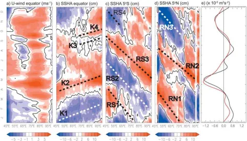
[23] Time-longitude diagrams of the zonal winds, sea surface height anomaly (SSHA) along the equator, along 5°S and 5°N, together with vertically integrated zonal pressure gradient and local acceleration terms are presented in Figures 8a – 8e. Note that the vertical integration is calculated over the depths where the EUC is defined. The zonal pressure gradient is calculated using centered differ-ences around 90°E with zonal separation of 8°(±4°around
Figure 6. (a) Eastward component of observed velocity from ADCP at 0°S, 90°E (shaded) superimposed on 15°C, 20°C, and 25°C isotherm depths from TRITON buoy at 1.5°S, 90°E (solid). Only values greater than 24 cm/s are shown for velocity with interval of 15 cm/s. (b) Time series of the EUC (vertically integrated zonal current from 90 to 170 m depth [black]) and surface zonal winds (red) averaged along the equator. (c) Time-depth section of the observed salinity at 1.5°S, 90°E. Note that all data have been smoothed with a 31-day running mean filter.
Table 2. Maximum Observed Eastward Velocity Component in the Thermocline And Depth Where the Undercurrent Was Observed
Date u(cm/s) Depth (m)
Boreal winter
26 April 2001 63 110
15 April 2002 91 110
2 April 2003 91 100
27 February 2004 85 120
15 April 2005 69 140
18 March 2006 74 110
Boreal summer
18 September 2001 34 130
9 October 2002 63 120
2003 The EUC was absent
2 November 2004 96 100
11 August 2005 64 160
9 November 2006a 96 70
a
The Indian Ocean Dipole (IOD) year.
90°E). Examination of the zonal pressure gradient using various ranges of the zonal separation, however, is hampered by the mooring location which is closed to the eastern boundary of the Indian Ocean.
[24] The major feature of the variations is undoubtedly semiannual variations. The easterly winds, which seem to be important for the development of eastward pressure gradient during boreal winter, initially are observed in Figure 7. (a) Squared coherency amplitude and (b) phase (in degree) between the equatorial zonal
winds and the EUC. Negative phase indicates that the zonal winds lead the EUC.
Figure 8. Time-longitude diagrams of (a) zonal winds along the equator, (b) SSHA along the equator, (c) SSHA along 5°S, and (d) SSHA along 5°N, together with (e) vertically integrated (90 – 170 m) zonal pressure gradient (red) and local acceleration (black) terms The pressure gradient is calculated using centered differences around 90°E with zonal separation of 8°.
December in the western basin (Figure 8a). As the oceanic response to the easterlies, the upwelling equatorial Kelvin waves are generated and propagated eastward across the basin approximately in one month (dashed line marked with ‘‘K1’’ in Figure 8b). Subsequently, the eastward pressure gradient is established with some delay to the wind-forcing (Figure 8e). By January – February, the regime of easterlies occupies most of the western and central equatorial regions and the eastward pressure gradient is fully developed. In addition, westward-propagating downwelling Rossby waves are reaching the western boundary by March and raising sea level in the west, contributing to the generation of the eastward pressure gradient (dashed line marked with ‘‘RS1’’ and ‘‘RN1’’ in Figures 8c – 8d).
[25] The upwelling Kelvin waves generated by easterly winds during December – January (dashed line marked with ‘‘K1’’ in Figure 8b) are reflected back to the interior Indian Ocean as a series of upwelling Rossby waves upon reaching the eastern boundary (dashed line marked with ‘‘RS2’’ in Figure 8c). On the other hand, the onset of the westerly winds in the eastern basin in late March (Figure 8a) excites equatorial Kelvin waves associated with downwelling in the equatorial waveguide (dashed line marked with ‘‘K2’’ in Figure 8b). Furthermore, the same westerly winds generate divergence in the off-equatorial region and this propagates westward as the upwelling Rossby waves, which also contribute to the low SSHA in the western part in April – May (Figure 8c). These sequences of events terminate the eastward pressure gradient and change its sign after May.
[26] During boreal summer, the downwelling Rossby waves radiated from the eastern boundary reach the western Indian Ocean by August – September lifting sea level there and, hence, generating the positive pressure gradient along the equator (dashed line marked with ‘‘RS3’’ and ‘‘RN2’’ in Figures 8c – 8d). Meanwhile, the equatorial upwelling Kelvin waves generated by weak easterly forcing in the central Indian Ocean reach the eastern boundary by August – September (dashed line marked with ‘‘K3’’ in Figure 8b). These sequences of events work together in generating subsurface eastward pressure gradient from July to September, although the latter contribution may be com-paratively weak during this season. By October, the down-welling Kelvin waves associated with westerly winds lift sea level in the eastern basin (dashed line marked with ‘‘K4’’ in Figure 8b). Subsequently, the eastward pressure gradient is decelerated (Figure 8e). In November, strong upwelling Rossby waves depressed the sea level in the western basin, helping to change the sign of pressure gradient (dashed line marked with ‘‘RS4’’ and ‘‘RN3’’ in Figures 8c–8d). Furthermore, the upwelling equatorial Kelvin waves, generated by the reflection of these upwelling Rossby waves upon reaching the western boundary, contribute to the initiation of the eastward pressure gradient during boreal winter (Figures 8b – 8e).
[27] It is important to note that the early study has demonstrated that basin-wide resonance is a possible forcing mechanism for the large amplitude semiannual variations in the equatorial Indian Ocean [Cane and Sarachik, 1981]. The resonance condition can be written asT=4L/(mcn), where
T is forcing period, Lthe basin width, cnthe speed of the
nth baroclinic vertical mode, andmthe positive integer. The resonance occurs when the traveltime for Kelvin waves and
the reflected first-meridional mode Rossby waves making a round trip of the basin is equal to the forcing period.Jensen
[1993] andHan et al.[1999] using numerical models have shown that resonant excitation of the second baroclinic vertical mode play an important role in strength and structure of equatorial currents. In particular,Han et al. [1999] have shown that the reflected Rossby waves from the eastern boundary accounted for the relatively large amplitude of semiannual response to the wind-forcing. More recently,Fu
[2007] has suggested that reflected Rossby waves from the western boundary also play a role in enhancing semiannual variations along the equatorial Indian Ocean.
[28] Although the wind-forcing could generate many modes in the observation as indicated by the upward phase propagation [McCreary, 1985], the geometry of the Indian Ocean basin is suitable for the second mode to be enhanced by the resonance mechanism at the semiannual timescale. Thus we argue that the resonance excitation at semiannual period may also contribute to the generation of semiannual eastward pressure gradient, which in turn has association with the subsurface eastward current. Note that model sensitivity experiments are required to quantify the contri-butions of the basin-wide resonance mechanism to the generation of the EUC in the Indian Ocean.
6. Anomalous Conditions During Boreal Summer of 2003 and 2006
[29] In addition to a strong seasonal variation, the tropical Indian Ocean also experiences significant interannual varia-tions associated with the Indian Ocean Dipole (IOD) and ENSO [Saji et al., 1999; Webster et al., 1999; Yu and Rienecker, 1999; Murtugudde et al., 2000]. In particular, the IOD event is inherent coupled ocean-atmosphere phe-nomenon in the tropical Indian Ocean that develops via feedbacks between zonal wind stress, sea surface temperature (SST) and thermocline depth anomalies. The positive IOD event is characterized by the cold SST and shallow thermo-cline depth anomalies in the southeastern tropical basin, accompanied by the warm SST and deep thermocline depth anomalies in the western tropical basin [Saji et al., 1999;
Webster et al., 1999]. The equatorial winds reverse direction from westerlies to easterlies during the peak phase of the positive IOD event. Thus we expect the strong EUC during the positive IOD event.
[30] In 2003, positive IOD started evolving in early boreal summer. The evolution of the IOD, however, was suddenly terminated by large instraseasonal disturbances in the atmosphere [Rao and Yamagata, 2004]. On the other hand, a strong positive IOD event took place during 2006 [Vinayachandran et al., 2007; Horii et al., 2008]. In this section, we will contrast the relative magnitudes and dura-tions of the anomalous condidura-tions of the EUC during boreal summer of 2003 to those during boreal summer of 2006.
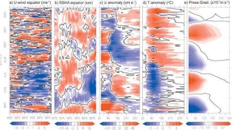
[31] Figures 9a – 9b shows the 2003 summer conditions of time-longitude sections of the zonal wind anomaly and SSHA along the equator, respectively. Time-depth sections of the zonal current anomaly at 0°S, 90°E, the temperature anomaly at 1.5°S, 9°0E and the zonal pressure gradient anomaly are presented in Figures 9c – 9e.
Kelvin waves were generated (Figures 9a – 9b). These upwelling Kelvin waves lowered the sea level in the east and strengthened the eastward pressure gradient in the upper layer down to the thermocline depth, leading to the eastward subsurface current in June – July (Figures 9c and 9e).
[33] In mid-August, anomalous westerly winds along the equator excited downwelling Kelvin waves and then readjusted the pressure gradient toward west (Figures 9a – 9b, 9e). The intensification of westerlies was interrupted by a short episode of the easterly winds in early September, which generated upwelling equatorial Kelvin waves (Figures 9a – 9b). This short episode of upwelling Kelvin waves together with an arrival of downwelling Rossby waves in the western boundary during August – September (not shown) counteracted the evolution of westward pressure gradient (Figures 9b, 9e). The incoming strong downwelling Kelvin waves in October, generated by westerly winds, lifted sea level in the eastern basin and enhanced the westward pressure gradient, which inhibited the eastward pressure gradient from continually developing (Figures 9a – 9b, 9e).
[34] It is worth noting that the temperature variations showed persistent positive anomaly from August to November (Figure 9d) and the current in the thermocline was anoma-lously westward from August to October (Figure 9c). We argue that this positive anomaly may play a role in the termination of the positive IOD event during 2003, in addition to the instraseasonal atmospheric disturbances suggested previously byRao and Yamagata[2004].
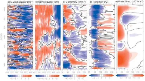
[35] During boreal summer-fall of 2006, in contrast, the equatorial winds underwent a dramatic reversal: anomalously strong easterly winds occupied most of equatorial region during this period (Figure 10a). The evolution of
anoma-lously strong and prolonged EUC initiated by anomalous easterlies that generated eastward pressure gradient in May (Figure 9). However, anomalously strong westerly winds were observed in late June and mid July, which excited strong downwelling equatorial Kelvin waves (Figures 10a – 10b). These together with upwelling Rossby waves reaching the western boundary in July (not shown) generated the westward pressure gradient (Figures 10b, 10e).
[36] In August, the easterly wind anomaly again intensi-fied in the central Indian Ocean (Figure 10a). The upwelling Kelvin waves associated with those easterly wind anomalies lowered sea level in the eastern basin (Figure 10b). At the same time, the downwelling Rossby waves, radiated from the eastern boundary, reached the western boundary and raised the sea level there (not shown). These sequences of events enhanced the eastward pressure gradient (Figure 10e). By September, the regime of easterlies occupied most of the equatorial region and persisted until the mooring was recov-ered in early December. These easterly winds seem to retain the eastward pressure gradient force, which results in a strong EUC during this period (Figures 10c and 10e).
[37] Corresponding changes were also observed in the tem-perature structure. The negative anomaly within the thermo-cline was observed from May until the end of the observation, which was interrupted by a short period of positive anomalies in early August and mid-September (Figure 10d). However, we cannot show the timing of the termination of EUC as it is still flowing when the mooring was recovered.
7. Summary and Discussion
[38] Characteristics of the subsurface eastward current, defined as EUC in the present study, in the eastern equatorial Figure 9. Time-longitude plots of (a) zonal winds anomaly along the equator, (b) SSHA along the
equator, together with time-depth variations of (c) zonal current anomaly at 0°S, 90°E, (d) temperature anomaly at 0°S, 90°E, and (e) zonal pressure gradient anomaly during May – November 2003.
Indian Ocean were investigated using an ADCP mooring data. Although the current was observed at a single point, it provides insight into the life cycle of the EUC from its genesis to its demises. In combination with recent TRITON buoy data, satellite observed SSH and surface winds and ARGO buoy data, we were able to examine generation mechanism of the EUC in the eastern equatorial Indian Ocean.
[39] The observed zonal currents reveal a robust EUC during both boreal winter and summer. We note that there is a decrease (an increase) in temperature (salinity) when the EUC is present. The presence of easterlies during boreal winter drives an upwelling Kelvin wave along the equator and a wind induced eastward pressure gradient excites flow in the thermocline to the east. During boreal summer, on the other hand, only weak easterly winds are observed along the equator leading to weak upwelling Kelvin waves. However, the reflection of downwelling Kelvin waves in the eastern boundary during boreal spring results in strong downwelling Rossby waves, which in turn play a significant role in generating eastward pressure gradient in summer.
[40] Our analysis shows that the equatorial waves play an important role for the generation of subsurface eastward pressure gradient that forces the EUC. However, Cane
[1980] has suggested the importance of nonlinearity in the dynamics of equatorial currents in the Indian Ocean. According to the Cane’s hypothesis, both easterly and westerly winds can generate the EUC through the mass adjustment. For easterly, the eastward pressure gradient that forces an undercurrent is driven directly by the easterly winds and indirectly through the meridional advection of vorticity. On the other hand, the westerly drives subsurface eastward flow through the downward advection of the
eastward momentum. Previous observational studies in the central Indian Ocean have suggested that the nonlinearity might be important in dynamics of Indian Ocean equatorial currents at thermocline depth [McPhaden, 1982; Nagura and McPhaden, 2008]. In particular,Nagura and McPhaden
[2008] noted that the nonlinearity effects were most impor-tant for the mean circulation but of secondary importance for seasonally varying depth-integrated zonal currents. The present analysis which is conducted on a single point, however, could not confirm the Cane’s hypothesis. Further analyses require data from a comprehensive observation or a high-resolution model simulation.
[41] It has been known that the intense westerly winds during the monsoon transition periods in April/May and October/November generate strong eastward oceanic jets in the upper layer as first reported byWyrtki[1973]. Previous studies have suggested that the jet is a basic upper ocean response to the semiannual westerly wind burst along the equatorial Indian Ocean [O’Brien and Hurlburt, 1974;Han et al., 1999]. Our observation shows that the Wyrtki jet in spring is slightly stronger that that in fall. The onset of westerly winds in spring and the induced spring Wyrtki jet terminate the eastward pressure gradient force which in turn reverse the eastward current in the thermocline (see Figure 8). Similarly, the fall Wyrtki jet also contributes to the termination of eastward pressure force which is previ-ously generated in summer.
[42] Moreover, we note that the EUC during boreal summer undergoes interannual variations. It was absent during 2003, while anomalously strong EUC existed throughout the latter half of 2006. This is attributed to the interannual modulation in easterly winds. During boreal summer of 2003, the equatorial winds were dominated by Figure 10. As in Figure 9 except during May – November 2006.
westerly winds that inhibited the formation of an eastward pressure gradient leading to the absence of the EUC. On the other hand, the winds remained easterly during the latter half of 2006, which maintain the eastward pressure gradient. Similar interannual variation in the EUC was also observed in the Pacific Ocean. Firing et al. [1983] have attributed the disappearance of the EUC during 1982/83 El Nin˜o to the collapse of the easterly trade winds during this period.Yu and McPhaden[1999] came to a similar conclusion that the interannual oceanic variations in the equatorial Pacific are in balance with the wind-forcing. Interplay of the IOD and the EUC in the Indian Ocean, however, remains unexplained and will be the subject of our future work.
[43] Acknowledgments. The authors would like to thank H. Hase, I. Ueki, and T. Horii for providing the ADCP and TRITON buoy data and to S. Hosoda for the ARGO data. We are also indebted to T. Tozuka for helpful comments on an earlier version of this article. This work has been supported by the Japan Society for Promotion of Science under Grant-in-Aid for Young Researcher (KAKENHI: 19.07606). The first author is supported by the Japan Society for the Promotion of Science through the postdoctoral fellowships for foreign researcher. The anonymous reviewers, whose helpful comments served to improve the article, are gratefully acknowledged.
References
Akima, H. (1970), A new method of interpolation and smooth curve fitting based on local procedures,J. Assoc. Comput. Mach.,17, 589 – 602. Bruce, J. G. (1973), Equatorial undercurrent in the western Indian Ocean
during the southwest monsoon,J. Geophys. Res.,78(27), 6386 – 6394. Cane, M. A. (1980), On the dynamics of equatorial currents, with application
to the Indian Ocean,Deep Sea Res. Part A,27, 525 – 544.
Cane, M. A., and E. S. Sarachik (1981), The response of linear baroclinic equatorial ocean to periodic forcing,J. Mar. Res.,39, 651 – 693. Firing, E., R. Lukas, J. Sadler, and K. Wyrtki (1983), Equatorial
under-current disappears during 1982 – 1983 El Nin˜o,Science,222, 1121 – 1122. Fu, L. L. (2007), Intraseasonal variability of the equatorial Indian Ocean observed from sea surface height, wind, and temperature data,J. Phys. Oceanogr.,37, 188 – 202.
Han, W., and J. P. McCreary (2001), Modeling salinity distributions in the Indian Ocean,J. Geophys. Res.,106, 859 – 877.
Han, W., J. P. McCreary, J. D. L. T. Anderson, and A. J. Mariano (1999), On the dynamics of the eastward surface jets in the equatorial Indian Ocean,J. Phys. Oceanogr.,29, 2191 – 2209.
Hase, H., Y. Masumoto, Y. Kuroda, and K. Mizuno (2008), Semiannual variability in temperature and salinity observed by Triangle Trans-Ocean Buoy Network (TRITON) buoys in the eastern tropical Indian Ocean,
J. Geophys. Res., 113, C01016, doi:10.1029/2006JC004026. Horii, T., H. Hase, I. Ueki, and Y. Masumoto (2008), Oceanic precondition
and evolution of the 2006 Indian Ocean dipole,Geophys. Res. Lett.,35, L03607, doi:10.1029/2007GL032464.
Hosoda, S., S. Minato, and N. Shikama (2006), Seasonal temperature var-iation below the thermocline detected by Argo floats,Geophys. Res. Lett.,
33, L13604, doi:10.1029/2006GL026070.
Jensen, T. G. (1993), Equatorial variability and resonance in a wind-driven Indian Ocean Model,J. Geophys. Res.,98, 22,533 – 22,552.
Knauss, J. A., and B. A. Taft (1964), Equatorial undercurrent of the Indian Ocean,Science,143, 354 – 356.
Knox, R. A. (1976), On a long series of measurements of Indian Ocean equatorial currents near Addu Atoll,Deep Sea Res.,23, 211 – 221. Kuroda, Y. (2002), TRITON: Present status and future plan,TOCS Rep.,
No. 5, 77 pp., JAMSTEC, Kanagawa, Japan. (Available at http:// www.jamstec.go.jp/jamstec/TRITON/future/index.html)
Masumoto, Y., H. Hase, Y. Kuroda, H. Matsuura, and K. Takeuchi (2005), Intraseasonal variability in the upper layer currents observed in the east-ern equatorial Indian Ocean, Geophys. Res. Lett., 32, L02607, doi:10.1029/2004GL021896.
McCreary, J. P. (1981), A linear stratified ocean model of the equatorial undercurrent,Philos. Trans. R. Soc.,A298, 603 – 635.
McCreary, J. P. (1985), Modeling equatorial ocean circulation,Annu. Rev. Fluid Mech.,17, 359 – 409.
McPhaden, M. J. (1982), Variability in the central equatorial Indian Ocean. Part I: Ocean dynamics,J. Mar. Res.,40, 157 – 176.
McPhaden, M. J., G. Meyers, K. Ando, Y. Masumoto, V. S. N. Murty, M. Ravichandran, F. Syamsuddin, J. Vialard, L. Yu, and W. Yu (2009), RAMA: The Research Moored Array for African-Asian-Australian mon-soon analysis and prediction,Bull. Am. Meteorol. Soc.,90, 459 – 480. Mizuno, K. (1995), Basin-scale hydrographic analysis and optimal
inter-polation method (in Japanese with English abstract),Oceanogr. Jpn.,4, 187 – 208.
Murtugudde, R. G., J. P. McCreary, and A. J. Busalacchi (2000), Oceanic processes associated with anomalous events in the Indian Ocean with relevance to 1997 – 1998,J. Geophys. Res.,105, 3295 – 3306. Nagura, M., and M. J. McPhaden (2008), The dynamics of zonal current
variations in the central Indian Ocean,Geophys. Res. Lett.,35, L23603, doi:10.1029/2008GL035961.
O’Brien, J. J., and H. E. Hurlburt (1974), Equatorial jet in the Indian Ocean: Theory,Science,184, 1075 – 1077.
Philander, S. G. H., and R. C. Pacanowski (1980), The generation of equatorial currents,J. Geophys. Res.,85, 1123 – 1136.
Rao, S. S., and T. Yamagata (2004), Abrupt termination of Indian Ocean dipole events in response to instraseasonal oscillations, Geophys. Res. Lett.,31, L19306, doi:10.1029/2004GL020842.
Reppin, J., F. A. Schott, J. Fischer, and D. Quadfasel (1999), Equatorial currents and transports in the upper central Indian Ocean: Annual cycle and interannual variability,J. Geophys. Res.,104, 15,495 – 15,514. Reverdin, G. (1987), The upper equatorial Indian Ocean: The climatological
seasonal cycle,Phys. Oceanogr.,17, 903 – 927.
Saji, N. H., B. N. Goswami, P. N. Vinayachandran, and T. Yamagata (1999), A dipole mode in the tropical Indian Ocean, Nature, 401, 360 – 363.
Schott, F., and J. P. McCreary (2001), The monsoon circulation of the Indian Ocean,Prog. Oceanogr.,51, 1 – 123.
Senan, R., D. Sengupta, and B. N. Goswami (2003), Intraseasonal ‘‘monsoon jets’’ in the equatorial Indian Ocean,Geophys. Res. Lett.,30(14), 1750, doi:10.1029/2003GL017583.
Stalcup, M. C., and W. G. Metcalf (1966), Direct measurements of the Atlantic Equatorial Undercurrent,J. Mar. Res.,24, 44 – 55.
Vinayachandran, P. N., J. Kurian, and C. P. Neema (2007), Indian Ocean response to anomalous conditions in 2006,Geophys. Res. Lett.,34, L15602, doi:10.1029/2007GL030194.
Webster, P. J., A. M. Moore, J. P. Loschnigg, and R. R. Leben (1999), Coupled ocean-atmosphere dynamics in the Indian Ocean during 1997 – 98,Nature,401, 356 – 359.
White, W. B. (1995), Design of global observing system for gyre-scale upper ocean temperature variability,Prog. Oceanogr.,36, 169 – 217. Wyrtki, K. (1973), An equatorial jet in the Indian Ocean,Science, 181,
262 – 264.
Yu, L., and M. Rienecker (1999), Mechanisms for the Indian Ocean warming during 1997 – 1998 El Nin˜o,Geophys. Res. Lett.,26, 735 – 738. Yu, X., and M. J. McPhaden (1999), Dynamical analysis of seasonal and
interannual variability in the equatorial Pacific,J. Phys. Oceanogr.,29, 2350 – 2369.
I. Iskandar, Y. Masumoto, and K. Mizuno, Institute of Observational Research for Global Change, Japan Agency for Marine-Earth Science and Technology, 2-15, Natsushima, Yokosuka, Kanagawa 237-0061, Japan. ([email protected])