Dynamics of wind
‐
forced intraseasonal zonal current variations
in the equatorial Indian Ocean
Iskhaq Iskandar
1,2and Michael J. McPhaden
1Received 3 December 2010; revised 14 March 2011; accepted 6 April 2011; published 28 June 2011.
[1]
This study examines the structure and dynamics of wind
‐
forced intraseasonal zonal
current variability in the equatorial Indian Ocean. We take advantage of a variety of
satellite and in situ data sets, including unprecedented 4
–
8 year
‐
long velocity time
series records from the Research Moored Array for African
‐
Asian
‐
Australian Monsoon
Analysis and Prediction (RAMA) program. Spectral analysis reveals prominent
intraseasonal zonal currents variations along the equator with periods of 30
–
70 days.
These oscillations are vertically in phase above the thermocline and propagate eastward
with the local zonal winds. In the thermocline, intraseasonal zonal velocity variations also
propagate eastward across a broad range of phase speeds expected for low baroclinic
equatorial Kelvin waves; amplitudes decrease with depth, with deeper levels leading those
near surface. Collectively, these results suggest that the near
‐
surface layer responds
directly to intraseasonal zonal wind stress forcing and that subsequently energy radiates
downward and eastward in the thermocline in the form of wind
‐
forced equatorial Kelvin
waves. In addition, intraseasonal zonal current variability on the equator is coherent
with off
‐
equatorial sea surface height fluctuations in the eastern and central of the basin.
This coherence is primarily due to the fact that equatorial zonal wind variations are
associated with off
‐
equatorial wind stress curls that can generate local Ekman pumping
and westward propagating Rossby waves.
Citation: Iskandar, I., and M. J. McPhaden (2011), Dynamics of wind‐forced intraseasonal zonal current variations in the equatorial Indian Ocean,J. Geophys. Res.,116, C06019, doi:10.1029/2010JC006864.
1.
Introduction
[2] An important aspect revealed from early observational studies in the tropical Indian Ocean is a pronounced intra-seasonal variability in zonal current velocity [McPhaden, 1982; Luyten and Roemmich, 1982; Reppin et al., 1999; Masumoto et al., 2005]. In the western equatorial region, zonal current data in the uppermost 200 m observed using an array of current meter moorings from 47° to 59°E during April 1979 to June 1980 showed a substantial intraseasonal variability at period of about 50 days [Luyten and Roemmich, 1982]. Early observational efforts in the central basin at Gan Island (73°10′E, 0°41′S) demonstrated the existence of 30–60 day variations in the zonal current [McPhaden, 1982]. He noted the apparent association with atmospheric vari-ability and found that intraseasonal zonal winds are coherent with intraseasonal zonal currents in the upper 100 m of the water column. Similarly, near‐surface zonal currents from current meter moorings in the central Indian Ocean (0°45′S– 5°N, 80°30′E) during July 1993 to September 1994 reveal
significant spectral energy at 40–60 day periods [Reppin et al., 1999]. Observations from Acoustic Doppler Current Profilers (ADCPs) moored at 0°S, 90°E, moreover, show dominant 30–50 day period variations in upper layer zonal currents down to 120 m depth [Masumoto et al., 2005]. Fu[2007] also found significant intraseasonal variability in altimeter derived SSH across a broad range of periods between 60 and 120 days with period bands theoretically in resonance with zonal wind forcing.
[3] Sengupta et al.[2001], using an ocean general circu-lation model forced with daily wind stress, suggested that oceanic instabilities play a role in generating some of the observed 30–50 day variability in the western Indian Ocean and in the equatorial region south and east of Sri Lanka. However, model simulations and data analysis byHan and McCreary[2001] and Han[2005] showed that most intra-seasonal variability in zonal currents along the equator away from the western boundary is directly wind forced. This conclusion applies both to variability in the 30–60 day period band and to an oceanic resonant response to weak wind forcing near 90 day periods. Moreover,Sengupta et al. [2007] have shown that 30–60 day variations of the zonal upper‐ocean currents at the equator are directly wind forced. [4] In the Pacific, intraseasonal oceanic variability has been suggested to play a role on the evolution of the El Niño Southern Oscillation (ENSO). For example, frequent strong intraseasonal westerly wind events are observed in the western 1
Pacific Marine Environmental Laboratory, NOAA, Seattle, Washington, USA.
2On leave from Jurusan Fisika, Fakultas Matematika dan Ilmu
Pengetahuan Alam, Universitas Sriwijaya, Palembang, Indonesia.
Copyright 2011 by the American Geophysical Union. 0148‐0227/11/2010JC006864
Pacific prior to El Niño [Luther et al., 1983]. Downwelling equatorial Kelvin waves are generated as a basic dynamical ocean response to these intraseasonal wind variations, which contribute to the initiation of El Niño events [Kessler et al., 1995; McPhaden and Yu, 1999]. The aforementioned scale interactions between intraseasonal and lower‐frequency phe-nomena have been suggested to occur in the tropical Indian Ocean [Han et al., 2006;Rao and Yamagata, 2004]. Episodic wind events on intraseasonal timescales during 1990s for example may have caused irregularity of the Indian Ocean Dipole (IOD), delaying the onset of 1997 IOD event by about 1 month relative to previous events [Han et al., 2006] and contributing to the early termination of the 1994 IOD event [Han et al., 2006]. Rao and Yamagata [2004] proposed a hypothesis about the role of intraseasonal variability in the termination of IOD events, given that strong intraseasonal winds occur in the equatorial Indian Ocean prior to the ter-mination of most IOD events. In particular, they suggested that downwelling Kelvin waves generated by intraseasonal westerlies deepen the thermocline and warm the sea surface temperature in the eastern equatorial Indian Ocean, leading to the termination of anomalous coupled air‐sea interactions.
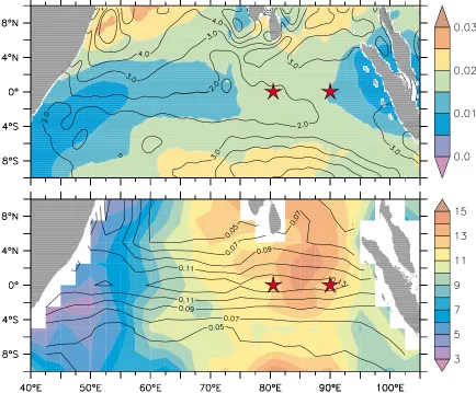
[5] Given the presumed importance of intraseasonal oce-anic variations on the evolution of seasonal and longer time scale coupled ocean‐atmosphere interactions in the tropical Indian Ocean, this study is intended to provide a compre-hensive description of the spatial and temporal character-istics of intraseasonal zonal currents in the 30–70 day period band along the equator in the Indian Ocean and to describe the dynamics underlying their development. We will rely primarily on in situ data from the Research Moored Array for African‐Asian‐Australian Monsoon Analysis and Pre-diction (RAMA) program [McPhaden et al., 2009] in com-bination with various other in situ and satellite data sets. The moored RAMA time series velocity data we use are unprecedented in length for the Indian Ocean, spanning nearly 8 years at one location (0°, 90°E) and nearly 4 years at another (0°, 80.5°E). The moorings are located zonally near maxima in intraseasonal variability for zonal currents, sea surface height, and atmospheric variability (Figure 1).
[6] The remainder of this paper is outlined as follow. Section 2 describes the data used in this study. Section 3 presents the seasonal and interannual characteristics of the observed variability. The temporal and spectral character-Figure 1. (top) Standard deviation of intraseasonal zonal wind stress (shaded, in N m−2) and sea surface
istics as well as vertical structures of intraseasonal vari-ability are presented in section 4. Section 5 discusses the forcing mechanisms for the intraseasonal variations. We summarize and discuss the broader relevance of these results in the final section.
2.
Data
[7] The data sets used in this study are listed in Table 1 and described below.
2.1. ADCP Data
[8] ADCP moorings in the equatorial Indian Ocean were implemented as part of the RAMA program to advance monsoon research and prediction. Moorings so far have been deployed along the equator at 80.5°E and 90°E (Figure 1). At 80.5°E, the ADCP data are processed to 5‐m vertical resolution with daily resolution from the surface down to 175 m depth for the period from 27 October 2004 to 17 October 2008. In this study we excluded the data shal-lower than 30 m depth as they might be contaminated by signals reflected at the surface. Early observed data from
this mooring site have been used to study the seasonal dynamics of upper equatorial zonal currents which showed an approximate balance between mean zonal wind stress and depth integrated pressure gradient on seasonal to interan-nual time scales, with small deviations from this balance due to wind‐forced equatorial wave dynamics [Nagura and McPhaden, 2008, 2010a, 2010b].
[9] ADCP moorings at 90°E provide daily current velocity data from surface down to 400 m depth with 10 m ver-tical resolution [Masumoto et al., 2005]. As at 80.5°E, we excluded data shallower than 40 m in depth because of surface backscatter contamination. In addition, we also neglected the data below 300 m, as they are very gappy in time [Iskandar et al., 2009]. The data are available for 14 November 2000 to 19 March 2009. Note that short gaps in the time series exist at both sites because of the time between mooring recoveries and redeployments. We have linearly interpolated across these gaps and other gaps shorter than 10 days resulting from instrument failure or other problems.
2.2. Subsurface Temperature and Salinity Data [10] In order to calculate density stratification, we used subsurface temperature and salinity data from Argo float observations provided by the Institut français de recherche pour l’exploitation de la mer (IFREMER) Coriolis data center. The data are available over a depth range of 5 to 1950 m with vertical resolution from 5 to 20 m for the upper 320 m. The data are mapped with a temporal resolution of 7 days on 0.5° × 0.5° horizontal grid though the effective horizontal resolution is closer to the Argo target of 3° × 3°. Quality control and mapping procedure for the temperature Table 1. Summary of Data Used in the Present Study
Data Interval Record Length
ADCP (0°, 90°E) daily 14 Nov 2000 to 19 Mar 2009 ADCP (0°, 80.5°E) daily 27 Oct 2004 to 7 Aug 2008 ARGO (T‐S) weekly Jan 2004 to Sep 2008 SSH (AVISO) weekly 14 Oct 1992 to 22 Jul 2009 QSCAT wind daily 1 Jan 2001 to 31 Dec 2008 OLR daily 1 Jan 2001 to 31 Dec 2008
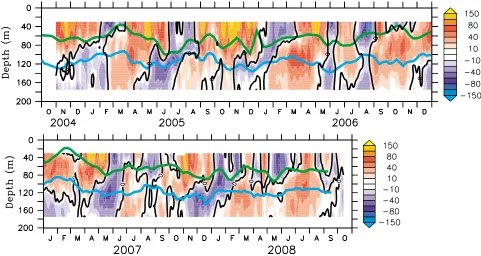
Figure 2. Time‐depth plot of zonal current at 0°S, 80.5°E. The data have been smoothed by 7‐day running mean filter. The eastward (westward) currents are shaded by reddish (bluish) color. The zero value is marked by the black contours. The green and blue curves show the 28°C and 20°C isotherms as a proxy for the top and bottom of the thermocline, respectively. These isotherms are calculated using weekly Argo data.
and salinity from Argo profiles are described inRoemmich and Gilson [2009]. The data are available for the period of January 2004 to September 2008.
2.3. Altimeter Data
[11] Sea surface height (SSH) data are obtained from Archiving, Validation and Interpretation of Satellite Ocean-ographic Data (AVISO) (http://www.aviso.oceanobs.com). This data set is merged data from all altimeter missions (Jason‐1 and 2, TOPEX/Poseidon, Envisat, and several other missions). The data set has a horizontal resolution of 0.25° × 0.25° and temporal resolution of 7 days and is available from 14 October 1992 to 22 July 2009. Note that long‐term means have been removed at each grid point to eliminate errors associated with uncertainties with the geoid.
2.4. Near‐Surface Currents
[12] We use near‐surface velocity data from the Ocean Surface Current Analysis‐Real time (OSCAR) project [Bonjean and Lagerloef, 2002], which is representative of flow at 15 m depth. This product is derived from satellite SSH, surface winds, and drifter data using a diagnostic model of ocean currents based on frictional and geostrophic dynamics. The data are available from 21 October 1992 to 1 September 2010 with horizontal resolution of 1° × 1° and temporal resolution of 5 days.
2.5. Surface Wind Data
[13] In order to evaluate dynamical forcing of the zonal transport variations, we make use of daily surface winds derived from the Quick Scatterometer (QSCAT). Here, data with a uniform horizontal resolution of 0.25° of 1 January 2001 to 31 December 2008 are used. The daily surface winds are used to compute surface wind stress using a constant drag coefficient (1.43 × 10⁻³) and air density (1.225 kg m−3) following Weisberg and Wang[1997].
2.6. Outgoing Longwave Radiation
[14] Daily average outgoing longwave radiation (OLR) data are obtained from the National Oceanic and Atmo-spheric Administration’s Climate Diagnostic Center (NOAA/ CDC) [Leibmann and Smith, 1996]. These data were recon-structed from National Center for Atmospheric Research (NCAR) archives by filling the gaps using temporal and spatial interpolation. Data are analyzed for the period of 1 January 2001 to 31 December 2008 with horizontal reso-lution of 2.5°.
3.
Seasonal and Interannual Variations
[15] In this section we briefly describe seasonal and interannual variations of the observed currents at 80.5°E and 90°E as background for a more focused discussion of intraseasonal variability. Seasonal variations associated with the spring and fall eastward equatorial jet dominate zonal current variations in the eastern and central Indian Ocean (Figures 2 and 3). Variations on this timescale have been found in historical data sets [Wyrtki, 1973; Knox, 1976; McPhaden, 1982;Reppin et al., 1999] as well as in numerical models [O’Brien and Hurlburt, 1974; Gent et al., 1983; Han et al., 1999]. Strong westerly winds over the equatorial Indian Ocean during monsoon transitions in April–May and
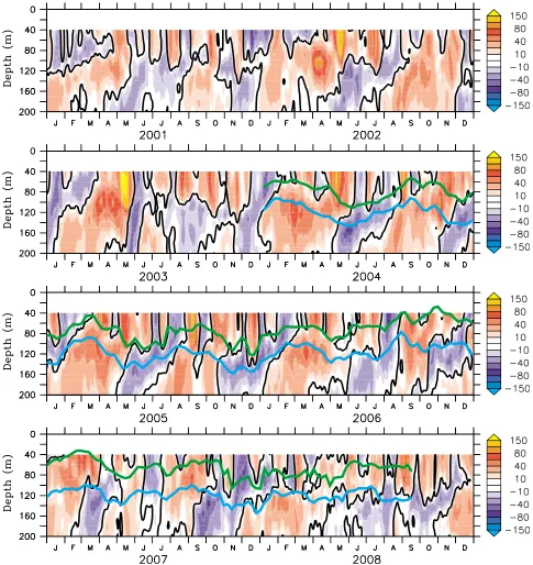
October–November force these eastward equatorial jets [Wyrtki, 1973;Han et al., 1999;Nagura and McPhaden, 2010a]. In the thermocline, semiannual eastward and west-ward subsurface currents are also present, although with phase shifted relative to those at the surface [McPhaden, 1982; Schott and McCreary, 2001; Iskandar et al., 2009] indicating downward propagation of wind forced energy. In addition, interannual variations are evident, such as the disappearance of fall jet during 2006 associated with the Indian Ocean Dipole (IOD) event [Horii et al., 2008;Nagura and McPhaden, 2010b].
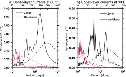
[16] In terms of spectral properties, observed currents and SSH clearly show spectral peaks at semiannual period (Figures 4a–4b). The sharpness of this peak, particularly at 90°E, compared to the energy at semiannual periods in zonal wind stress, has been attributed to a resonant equatorial mode [Jensen, 1993;Han et al., 1999]. Distinct annual variability is also revealed in the spectra of SSH (Figure 4b), zonal wind stress at 90°E, and OLR (Figures 4c–4d), but not in zonal currents at the mooring locations (Figure 4a).
[17] In contrast to zonal current spectra, meridional cur-rent spectra exhibit very little energy at periods longer than about 30 days at the mooring locations (Figures 5a–5b). This result is consistent with that ofMcPhaden[1982] who found a similar anisotropy in near surface currents from time series at 0°, 73°E. Such anisotropy is expected from the theory for low frequency (i.e., periods > 30 days) fluctua-tions in the equatorial waveguide. In contrast, there is much greater energy in meridional velocity at periods shorter than 20 days. Where“biweekly”fluctuations, with periods between 10 and 20 days, dominate meridional velocity var-iability. This result is consistent with earlier analyses in the central Indian Ocean, which reported dominant biweekly oscillation in the meridional velocity field [Reppin et al., 1999]. Recent studies have suggested that this biweekly variability is due to wind‐forced Yanai waves [Sengupta et al., 2004;Miyama et al., 2006].
4.
Intraseasonal Variations
4.1. Temporal and Spectral Characteristics
results from a wind‐forced basin‐mode resonance [Cane and Moore, 1981]. However, energy in the 90‐day period band is less prominent than at 30–70 days, particularly when viewed against a red noise background. As mentioned above, there also is virtually no energy in meridional velocity at periods longer than 30 days.
[20] Intraseasonal variations in the atmospheric quantities (zonal wind stress and OLR) are skewed to the higher high‐ frequency end of the intraseasonal band (Figures 4c–4d). Zonal wind and OLR spectra for example peak at periods around 30–50 days (Figure 4c). There is significant atmo-spheric energy at periods shorter than 30 days, but there is
little energy in zonal current and SSH at these periods. This “red shift”in the ocean response spectrum to intraseasonal atmospheric forcing can be rationalized in terms of a low‐ frequency–wave number scale selective oceanic Kelvin wave response to zonal wind stress forcing [Kessler et al., 1995;Hendon et al., 1998;Han, 2005].
4.2. Vertical Structures
[21] In order to describe the vertical structure of the intraseasonal zonal currents in the equatorial Indian Ocean, we use a complex empirical orthogonal function (CEOF) analysis. The CEOF analysis is a multivariate technique Figure 3. Same as Figure 2 except for the zonal current at 0°S, 90°E.
designed to obtain the dominant spatial patterns of vari-ability in a statistical field, providing amplitude and phase information in particular frequency bands [Horel, 1984]. The observed zonal currents have been decomposed into CEOF analysis using frequency band 0.014–0.035 cpd, that is, periods between about 29 and 71 days.
[22] The first three modes of CEOF at 80.5°E account for almost 95% of the total variance, of which the first mode accounts for 73.6% while the second and the third modes account for 13.2% and 8.1%, respectively. Similarly, at 90°E the three leading CEOF modes retain about 90% of the total zonal current variance, with the first mode cap-turing 70.2% of the total variance and the second and third modes contributing 13.0% and 6.9%, respectively. Since the first mode dominates most of the variability, we focus dis-cussion on this mode hereafter.
[23] The reconstructed time evolution of the first mode for intraseasonal zonal velocity at 80.5°E and 90°E are pre-sented in Figures 6 and 7, respectively. At 80.5°E, the time series shows a nearly constant phase in the vertical, though there is a gradual phase shift in depth with a tendency for deeper levels to lead those near surface (Figure 6). The reconstructed time series also indicates largest amplitude variability above 120 m depth. The reconstructed time series of the first CEOF mode at 90°E (Figure 7) shows a clearer vertical phase shift compared to that at 80.5°E (Figure 6).
[24] To be more quantitative, we calculate the upward phase propagation for the first CEOF mode at each site using a lag correlation analysis between the mean thermo-cline depth and the deepest depth at which mooring data available. The depth of the thermocline is estimated as the depth of 20°C isotherm, which is about 120 m on average at both mooring sites. The highest correlation coefficient at each depth relative to this depth is then plotted in a time‐
depth diagram. A linear least squares fit is applied to these coefficients and vertical phase speed is calculated from the slope of the line. The 95% confidence limits are obtained from procedures described byEmery and Thomson[2004] for trend analysis.
[25] The resulting phase speeds are 2.19 ± 1.48 × 10⁻⁴m s−1 at 80.5°E and 1.38 ± 0.29 × 10⁻⁴m s−1at 90°E. Following Kessler and McCreary [1993] and assuming the vertical propagating signal is a Kelvin wave, we may estimate its horizontal phase speed using the WKB approximation. The characteristic speed is given asc= N/∣m∣, whereNdenotes the Brunt‐Väisälä frequency andmindicates a local vertical wave number. In our analysis the local vertical wave number is estimated from the calculated upward phase speed at each mooring site periods of 30–70 days. The resultant local wave numbers range from 4.74 × 10⁻³m−1to 11.07 × 10⁻³m−1at 80.5°E and 7.53 × 10⁻³m−1to 17.57 × 10⁻³m−1 at 90°E, respectively. These wave numbers correspond to vertical wavelength of 567.59 m to 1325.57 m and 357.61 m to 834.42 m, respectively.
[26] To estimate horizontal phase speed, we computed the meanNaveraged between the mean thermocline depth and the depth of the deepest current data available at each mooring site. For a background Brunt‐Väisälä frequency of 1.44 × 10⁻²s−1(at 80.5°E) and 1.31 × 10⁻²s−1(at 90°E), we obtained phase speedscof 1.30–3.04 m s−1and 0.75– 1.74 m s−1, respectively. These estimated phase speeds do not correspond to one particular baroclinic mode, though they fall within the range expected for the first three baroclinic modes (e.g.,c1= 2.5 m s−1,c2= 1.55 m s−1, andc3= 0.99 m s−1)
in the Indian Ocean [Nagura and McPhaden, 2010a]. [27] McCreary [1984] suggested that wind forced equa-torial Kelvin waves would propagate energy downward and phase upward and that this vertical propagation could be Figure 5. Same as Figure 4a except for the zonal (black) and meridional (red) currents averaged over
40–100 m depth at (a) 80.5°E and (b) 90°E. Note that scale is different in Figures 5a and 5b.
represented by the sum of vertical modes. In the forcing region the different vertical modes are phase locked, but they begin to disperse as they propagate eastward, with the lower modes traveling fastest. This dispersion may explain why the vertical phase shift is more apparent at 90°E than that at 80.5°E. A similar evolution of the vertical structure for equatorial intraseasonal Kelvin waves has been observed along the equator in the Pacific Ocean, indicating that more than one vertical mode is involved in the response to zonal wind‐forcing and that wind forced Kelvin wave energy propagates down and to the east [Kutsuwada and McPhaden, 2002].
[28] Further insight into the relationship between the intraseasonal zonal currents observed at both mooring sites is gained by calculating lag correlation between the time series of reconstructed zonal currents at 80.5°E and those at 90°E (Figure 8). A level‐by‐level correlation analysis indi-cates a gradual increase in time lag between intraseasonal signals at 80.5°E and those at 90°E when moving down-ward. Near the surface, the signals take only about 1–3 days to propagate from 80.5°E to 90°E, while below 100 m depth there is a lag of about 5–7 days. Thus the eastward propa-gation along the equator near the surface is much faster than in the thermocline. Indeed, the mean eastward phase speed of the 40–100 m intraseasonal zonal currents and its 90% confidence limits are 8.35 ± 2.62 m s−1as calculated from lag correlation presented in Figure 8. This phase speed is much higher than expected for free equatorial Kelvin waves in the equatorial Indian Ocean. However, one does not expect to see propagation at free Kelvin wave phase speeds in the surface layer when local wind forcing is prominent [Philander and Pacanowski, 1981;Roundy and Kiladis,
2006;Shinoda et al., 2008]. These results require an eval-uation of the forcing mechanisms for the intraseasonal variability, which we turn to in the following section.
5.
Forcing Mechanism
5.1. Surface Layer Versus Thermocline Response [29] Previous studies have suggested that intraseasonal zonal currents in the equatorial Indian Ocean result pri-marily from direct wind forcing [Han, 2005;Masumoto et al., 2005]. In order to better understand the dynamical forcing of the intraseasonal zonal currents in the equatorial Indian Ocean, we examine the relationship between the intraseaso-nal zointraseaso-nal wind stress and the zointraseaso-nal currents in this section.
[30] Correlations between the CEOF reconstructed zonal currents averaged over 40–100 m depth with the local intraseasonal zonal wind stress at both mooring sites indi-cates a virtually in phase relationship between the winds and the currents (Figures 9a and 9c). This in phase relation sug-gests a direct influence of wind stress forcing on the upper ocean at these time scales. Eastward phase speed of the surface currents along the equator as described in the previ-ous section is in fact comparable to that of the zonal wind stress forcing. Zonal winds propagate eastward along the equator at 8.74 ± 1.73 m s−1as computed from an amplitude‐ weighted linear least square fit of the maximum lagged correlation between stress at 60°E and 95°E (Figure 10a), with 90% confidence limits determined followingEmery and Thomson[2004]. Using similar procedures, we estimated the eastward propagation of atmospheric intraseasonal variability in OLR (Figure 10b) as 6.43 ± 2.29 m s−1. These eastward phase speeds for zonal winds and OLR are somewhat faster Figure 6. Reconstructed time series of the first CEOF mode for the intraseasonal zonal currents at 0°S,
than the roughly 5 m s−1 phase speeds expected for the Madden‐Julian Oscillation (MJO), which is the dominant mode of atmospheric intraseasonal variability over the Indian Ocean [Zhang, 2005]. The discrepancy may be related to sensitivities in the way we have computed phase speed, given the uncertainties in our estimates. It could also be that our method of phase speed estimation for winds and OLR includes other forms of intraseasonal variability besides the MJO. Nonetheless, we surmise that the MJO‐related forcing is largely responsible for the variability we observe in intra-seasonal zonal currents along the equator.
[31] Further insight into that nature of wind forcing on upper‐ocean intraseasonal zonal currents can be gained by examining the coherence and phase spectra between the zonal wind stress and the depth‐averaged (40–100 m) zonal currents at 80.5°E and those at 90°E for the 30–70 day
period band (Figure 11). As expected, the results show nearly in‐phase coherence between the zonal currents and zonal winds within ±10° of longitude at both mooring sites (Figures 11a–11b). Zonal currents at 80.5°E are signifi-cantly coherent with zonal wind stress between about 55°E and 85°E (Figure 11c), while those at 90°E show significant coherence with zonal wind stress between roughly 60°E and 90E (Figure 11d). Thus at each location the most effective winds at forcing the near surface layer are those that lie to the west of the mooring locations. These results, combined with those of the section 4, suggest that zonal currents in the near surface layer respond directly and rap-idly to eastward propagating intraseasonal zonal wind stress forcing, most likely related to the MJO, with energy radi-ating downward and eastward into the thermocline as remotely forced Kelvin waves.
Figure 7. Same as Figure 6 except for the reconstructed time series of the first CEOF mode at 0°S, 90°E.
5.2. Spatial and Temporal Evolution
[32] In order to illustrate the evolution of the oceanic variations in relation to the spatial structure of the intrasea-sonal atmospheric forcing, maps are constructed by
regres-sing intraseasonal wind stress, OLR, and SSH onto the corresponding CEOF reference time series of zonal currents at 0°, 90°E for different lags. The reference time series is generated from the depth‐averaged intraseasonal zonal Figure 8. Correlation coefficients for the reconstructed time series of the first CEOF mode of the
intraseasonal zonal currents between 90°E and 80.5°. The data for the period of 27 October 2004 to 17 October 2008 are used for the calculation. Note that positive (negative) lag means that the signal at 90°E leads (lags) that at 80.5°E. Correlations above 95% confidence limit are contoured.
currents from 40 to 100 m. Results do not depend sensi-tively on specific choice of the depth‐averaged, since other choices (e.g., 100–150 m and 40–150 m) yield similar results. In addition, regression onto zonal currents at 0°, 80.5°E yields similar results.
[33] The coherent evolution between OLR and surface wind anomalies (Figure 12) indicates that suppressed con-vection (positive OLR anomalies) is associated with easterly anomalies, while westerly wind anomalies are dominant in
regions of enhanced convection (negative OLR anomalies). Enhanced convection first appears over the eastern half of the basin at lag −14 days associated with a weakening of easterly winds and development of westerly winds (Figure 12c). This is followed by further development of convection and appearance of westerly winds (Figure 12d). The enhanced convection gradually moves eastward as shown in Figures 12c–12e. At zero lag when westerly winds are strong over the equatorial Indian Ocean, maximum
Figure 11. (a–b) Coherent amplitude and (c–d) phase between zonal wind stress along the equator and depth‐averaged (40–100 m) zonal currents at 80.5°E (Figures 11a and 11c) and that at 90°E (Figures 11b and 11d) in the intraseasonal period band (30–70 days). Positive (negative) phase lag indicates that the zonal wind stress leads (lags) the zonal currents. Gray shading indicates one standard error. Dashed lines in Figures 11a–11b indicate 90% confidence limits for the coherence, which is estimated as g95%= 1−(0.05)[2/(DOF− 2)][Emery and Thomson, 2004] and is equal to 0.58.
Figure 10. (a) Correlation between intraseasonal zonal wind stress at 90°E and at other longitudes along the equator. (b) Same as in Figure 10a except for the intraseasonal OLR. Correlations above 90% confi-dence limit are contoured. The solid blue line is a linear regression fit to time lag between 60°E and 95°E (Figure 10a) and 47.5°E and 95°E (Figure 10b).
convective anomalies have propagated further eastward (Figure 12e). Evolution and eastward propagation of sup-pressed convection is shown over the next couple of weeks (Figures 12f–12h). The evolution of suppressed convection
is associated with the weakening of westerly winds and the development of easterly winds over the eastern Indian Ocean. This coherent evolution of OLR and surface wind anomalies is consistent with the classical relationships for Figure 12. Maps of intraseasonal sea surface height (shading), OLR (contour), and wind stress (arrows)
regressed onto depth‐averaged (40–100 m) intraseasonal zonal currents at 0°, 90°E for lags between
these two variables on intraseasonal time scales described byRui and Wang’s [1990] analysis of the MJO.
[34] The SSH response to intraseasonal wind forcing indi-cates the presence of wind‐forced equatorially trapped waves near the equator. Easterly (westerly) winds are associated with depressed (elevated) sea levels beneath and to the east of the forcing region (e.g., Figures 12a and 12b and Figures 12e and 12f). These SSH patterns propagate eastward and, upon
reaching the west coast of Sumatra, propagate poleward both north and south of the equator as would be expected for coastal Kelvin waves (Figures 12e, 12f, and 12g). We also find that zonal surface current variations are trapped within several degrees of the equator (Figure 13). Elevated (depressed) sea levels along the equator are coherent with eastward (westward) surface currents consistent with the relationship expected for the wind‐forced Kelvin waves (Figure 13). Moreover, there Figure 13. Maps of intraseasonal (a) wind stress (arrows), OLR (contour), and sea surface height
(shading) regressed onto depth‐averaged (40–100 m) intraseasonal zonal currents at 0°, 90°E at zero lag (repeated from Figure 12e). (b) Same as in Figure 13a except for intraseasonal OSCAR surface currents (arrows) superimposed on sea surface height (shading).
Figure 14. Lagged regression of intraseasonal Ekman pumping (contour, negative downward in unit of m d−1) and sea surface height (shading, centimeters) with the depth‐averaged (40–100 m) intraseasonal zonal currents at 90°E averaged along (a) 3°–5°N and (b) 3°–5°S. Regressions are shown only where significant at 95%.
are suggestions of flow circulating around the sea level extrema along 4°N, as expected from geostrophy.
[35] Figure 12 also suggests the presence of westward propagating, low baroclinic mode Rossby waves in the lat-itude band centered near 4°N and 4°S. Some of this Rossby wave energy is boundary generated (as in Figures 12f–12g). However, these boundary‐generated features do not appear to propagate far offshore (Figure 14), perhaps because they are also radiating energy into the deep ocean consistent with ray theory for reflected waves [e.g.,McCreary, 1984]. Downward energy propagation of the reflected Rossby waves has been shown in a numerical study of intraseasonal variations in the equatorial Indian Ocean [Han, 2005].
[36] In contrast, SSH extrema centered along 4°N and 4°S between 70° and 90°E (Figures 12b and 12c and Figures 12f and 12g) may result from a combination of direct wind stress curl‐generated Ekman pumping (= r × (~
f), where
~
is wind stress, fis the Coriolis parameter, andris water density) and subsequent Rossby wave propagation in the interior ocean. Intraseasonal zonal wind stress forcing is strongest between 75° and 90°E (Figure 1) coincident with the longitude range of strongest Ekman pumping averaged between 3°–5°N and 3°–5°S (Figure 14). In the Northern Hemisphere, positive SSH signals in the central basin are preceded by downward (negative) Ekman pumping and negative SSHs are preceded by upward (positive) Ekman pumping, with the peak SSH signals located just west of the peak Ekman pumping. There tends to be symmetry around the equator in both forcing and response, though the oceanic response is somewhat less clearly defined in the Southern Hemisphere. The westward progression of SSH relative to the Ekman pumping forcing suggests a Rossby wave com-ponent to the response. However, energy does not appear to penetrate far to the west of the forcing, perhaps because it also radiates into the deep ocean. It is also possible that weak Ekman pumping of opposite sign to that east 70°E may contribute to the disappearance of the Rossby wave signals in the central and western basin.
[37] Finally, we note that the connection between intra-seasonal currents on the equator at 90°E and off‐equatorial sea level variations further to the west (Figures 12–14) is mediated by a commonality in wind forcing. Associated with zonal wind stress variations that drive zonal currents on the equator is a wind stress curl pattern (evident in the meridional shear of zonal winds in Figure 12e) that leads to local horizontal convergence and divergence of mass. Local changes in mass are reflected in sea level variations, which tend to radiate westward in the form of equatorial Rossby waves. These interior ocean changes are in addition to those that result from the reflection of Kelvin waves into Rossby waves at the eastern boundary.
6.
Summary and Discussion
[38] Intraseasonal zonal currents in the equatorial Indian Ocean are investigated using ADCP data moored along the equator at 80.5°E and 90°E as well as other satellite and in situ data sets. Spectral analysis shows that intraseasonal zonal currents at both mooring sites are characterized by prominent 30–70 day variations. The vertical structures of these intraseasonal signals are evaluated using a CEOF analysis, with the first CEOF mode at 80.5°E and 90°E
accounting for 73.6% and 70.2% of the total zonal current variance, respectively. At both mooring sites, largest vari-ability is observed in the upper 100 m above the thermo-cline, while within the thermothermo-cline, amplitudes decrease with depth.
[39] The vertical structures of the intraseasonal zonal currents reconstructed from first CEOF mode at both mooring sites are vertically in phase above the thermocline. On the other hand, in the thermocline we found a gradual phase shift with a tendency for the deeper levels to lead those near surface, with the phase shift more apparent at 90°E than 80.5°E. The horizontal phase speed estimated using the WKB approximation based on the first CEOF mode and observed density profiles reveals that the signals propagate eastward with phase speeds fall within the range expected for the first three baroclinic modes in the Indian Ocean [Nagura and McPhaden, 2010a]. According to linear wave theory, wind forced equatorial Kelvin waves would propagate energy downward and phase upward. This vertical propagation can be represented mathematically by the sum of vertical modes [McCreary, 1984]. In the presence of forcing, the different vertical modes are phase locked, but they begin to disperse as they propagate eastward, with the lower modes traveling faster. This dispersion may explain why the vertical phase shift is more apparent at 90°E than that at 80.5°E.
[40] A level‐by‐level analysis of the correlation functions indicates a gradual increase in time lag between intrasea-sonal signals at 80.5°E and those at 90°E when moving downward, implying that eastward propagation along the equator near the surface is much faster than in the thermo-cline. The correlation analysis between the local intrasea-sonal zonal wind stress and the reconstructed zonal currents averaged over 40–100 m depth from the first CEOF mode at both mooring sites shows that there is an in phase rela-tionship between the local zonal wind stress forcing and the zonal current above the thermocline. On the other hand, in the thermocline, correlation between the local zonal wind stress forcing and the reconstructed zonal currents indicates an increase in time lag between two with zonal wind cur-rents leading the zonal wind stress at both locations. These results suggest that the zonal currents in the near surface layer respond directly and rapidly to local intraseasonal zonal wind stress forcing, with energy radiating downward and eastward into the thermocline as remotely forced Kelvin waves. Given the structure of atmospheric variability asso-ciated with the zonal current fluctuations on intraseasonal time scales, we infer that MJO‐related variability is the most likely source of wind forcing.
as westward propagating Rossby waves. However, these boundary‐generated Rossby waves do not appear to propagate far offshore, perhaps because they are radiating into the deep ocean as would be expected from ray theory for reflected waves. In addition, off‐equatorial SSH variability in the inte-rior of the basin between 70°E and 90°E appears to be influ-enced on intraseasonal time scales by local Ekman pumping and Rossby wave dynamics.
[42] The role of Rossby waves on the intraseasonal oce-anic variations along the equator has been discussed in previous studies. For example, Fu [2007] suggested that there is a resonant excitation of the second baroclinic mode by 60‐day zonal winds, in which reflected Rossby waves from the eastern boundary reinforce direct wind‐forced Kelvin waves. Han[2005] suggested that reflected Rossby waves within 30–60‐day period band significantly contrib-ute to variations in deeper layers of the thermocline, con-sistent with our results suggesting significant downward energy propagation at these periods in the thermocline.
[43] We note significant energy at period of about 90‐day in the observed zonal currents and SSH in addition to prominent 30–70 day variation.Han[2005] suggested that this 90‐day peak is a selective response of the ocean to the weak 90‐day wind variations involving a resonant basin mode as described by Cane and Moore [1981]. Detailed study of the dynamics and structures of the observed 90‐day zonal currents is an important part of our ongoing research and will be reported at a later time.
[44] Acknowledgments. We thank Iwao Ueki of JAMSTEC for
providing 90°E ADCP data. The Coriolis data center provided the gridded temperature and salinity data set. The gridded SSH data are provided by the Ssalto/Duacs multimission altimeter project (http://www.aviso.oceanobs. com/) and the QSCAT data are provided by the Remote Sensing System (www.remss.com/data/qscat). We also thank T. Tozuka for providing CEOF code and A. Santoso for providing the red‐noise Matlab code. The authors are indebted to Motoki Nagura for useful discussions during the course of this work. Constructive comments by two anonymous reviewers helped improved the original draft of this paper. The first author is supported by the National Research Council through the Research Associateships Program. This is PMEL contribution 3645.
References
Bonjean, F., and G. S. E. Lagerloef (2002), Diagnostic model and analysis of the surface currents in the tropical Pacific Ocean,J. Phys. Oceanogr.,32, 2938–2954, doi:10.1175/1520-0485(2002)032<2938:DMAAOT>2.0. CO;2.
Cane, M., and D. W. Moore (1981), A note on low‐frequency equatorial basin modes,J. Phys. Oceanogr.,11, 1578–1584, doi:10.1175/1520-0485(1981)011<1578:ANOLFE>2.0.CO;2.
Emery, W. J., and R. E. Thomson (2004),Data Analysis Methods in Physical Oceanography, Elseiver, Amsterdam.
Fu, L. L. (2007), Intraseasonal variability of the equatorial Indian Ocean observed from sea surface height, wind, and temperature data,J. Phys. Oceanogr.,37, 188–202, doi:10.1175/JPO3006.1.
Gent, P. R., K. O’Neill, and M. A. Cane (1983), A model of the semi-annual oscillation in the equatorial Indian Ocean,J. Phys. Oceanogr., 13, 2148–2160, doi:10.1175/1520-0485(1983)013<2148:AMOTSO>2.0. CO;2.
Han, W. (2005), Origins and dynamics of the 90‐day and 30–60‐day variations in the equatorial Indian Ocean,J. Phys. Oceanogr.,35, 708–728, doi:10.1175/JPO2725.1.
Han, W., and J. P. McCreary (2001), Modeling salinity distributions in the Indian Ocean,J. Geophys. Res.,106, 859–877, doi:10.1029/2000JC000316. Han, W., J. P. McCreary, J. D. L. T. Anderson, and A. J. Mariano (1999), On the dynamics of the eastward surface jets in the equatorial Indian Ocean,J. Phys. Oceanogr.,29, 2191–2209, doi:10.1175/1520-0485 (1999)029<2191:DOTESJ>2.0.CO;2.
Han, W., T. Shinoda, L.‐L. Fu, and J. P. McCreary (2006), Impact of atmo-spheric intraseasonal oscillations on the Indian Ocean dipole during the 1990s,J. Phys. Oceanogr.,36, 670–690, doi:10.1175/JPO2892.1. Hendon, H., B. Liebmann, and J. D. Glick (1998), Oceanic Kelvin waves
and the Madden‐Julian oscillation,J. Atmos. Sci.,55, 88–101, doi:10.1175/1520-0469(1998)055<0088:OKWATM>2.0.CO;2. Horel, J. D. (1984), Complex principal component analysis: Theory and
examples,J. Clim. Appl. Meteorol.,23, 1660–1673, doi:10.1175/1520-0450(1984)023<1660:CPCATA>2.0.CO;2.
Horii, T., H. Hase, I. Ueki, and Y. Masumoto (2008), Oceanic precondition and evolution of the 2006 Indian Ocean dipole,Geophys. Res. Lett.,35, L03607, doi:10.1029/2007GL032464.
Iskandar, I., Y. Masumoto, and K. Mizuno (2009), Subsurface equatorial zonal current in the eastern Indian Ocean,J. Geophys. Res.,114, C06005, doi:10.1029/2008JC005188.
Jensen, T. G. (1993), Equatorial variability and resonance in a wind‐driven Indian Ocean model,J. Geophys. Res.,98, 22,533–22,552, doi:10.1029/ 93JC02565.
Kessler, W. S., and J. P. McCreary (1993), The annual wind‐driven Rossby wave in the subthermocline equatorial Pacific,J. Phys. Oceanogr.,23, 1192–1207, doi:10.1175/1520-0485(1993)023<1192:TAWDRW>2.0. CO;2.
Kessler, W. S., M. J. McPhaden, and K. M. Weickmann (1995), Forcing of intraseasonal Kelvin waves in the equatorial Pacific,J. Geophys. Res., 100, 10,613–10,631, doi:10.1029/95JC00382.
Knox, R. A. (1976), On a long series of measurements of Indian Ocean equatorial currents near Addu Atoll,Deep Sea Res.,23, 211–221. Kutsuwada, K., and M. J. McPhaden (2002), Intraseasonal variations in the
upper equatorial Pacific Ocean prior to and during the 1997–98 El Niño, J. Phys. Oceanogr.,32, 1133–1149, doi:10.1175/1520-0485(2002) 032<1133:IVITUE>2.0.CO;2.
Leibmann, B., and C. A. Smith (1996), Description of a complete (interpo-lated) outgoing longwave radiation dataset,Bull. Am. Meteorol. Soc.,77, 1275–1277.
Luther, D. S., D. E. Harrison, and R. A. Knox (1983), Zonal winds in the central equatorial Pacific and El Niño,Science,222, 327–330, doi:10.1126/ science.222.4621.327.
Luyten, J. R., and D. H. Roemmich (1982), Equatorial currents at semi‐ annual period in the Indian Ocean,J. Phys. Oceanogr.,12, 406–413, doi:10.1175/1520-0485(1982)012<0406:ECASAP>2.0.CO;2.
Masumoto, Y., H. Hase, Y. Kuroda, H. Matsuura, and K. Takeuchi (2005), Intraseasonal variability in the upper layer currents observed in the eastern equatorial Indian Ocean,Geophys. Res. Lett.,32, L02607, doi:10.1029/ 2004GL021896.
McCreary, J. P. (1984), Equatorial beams,J. Mar. Res.,42, 395–430, doi:10.1357/002224084788502792.
McPhaden, M. J. (1982), Variability in the central equatorial Indian Ocean. Part I: Ocean dynamics,J. Mar. Res.,40, 157–176.
McPhaden, M. J., and X. Yu (1999), Equatorial waves and the 1997–98 El Niño,Geophys. Res. Lett.,26, 2961–2964, doi:10.1029/1999GL004901. McPhaden, M. J., G. Meyers, K. Ando, Y. Masumoto, V. S. N. Murty, M. Ravichandran, F. Syamsuddin, J. Vialard, L. Yu, and W. Yu (2009), RAMA: The Research Moored Array for African‐Asian‐Australian mon-soon analysis and prediction,Bull. Am. Meteorol. Soc.,90, 459–480, doi:10.1175/2008BAMS2608.1.
Miyama, T., J. P. McCreary, D. Sengupta, and R. Senan (2006), Dynamics of biweekly oscillations in the equatorial Indian Ocean,J. Phys. Ocea-nogr.,36, 827–846, doi:10.1175/JPO2897.1.
Nagura, M., and M. J. McPhaden (2008), The dynamics of zonal current variations in the central Indian Ocean,Geophys. Res. Lett.,35, L23603, doi:10.1029/2008GL035961.
Nagura, M., and M. J. McPhaden (2010a), Wyrtki Jet dynamics: Seasonal variability,J. Geophys. Res.,115, C07009, doi:10.1029/2009JC005922. Nagura, M., and M. J. McPhaden (2010b), Dynamics of zonal current var-iations associated with the Indian Ocean dipole,J. Geophys. Res.,115, C11026, doi:10.1029/2010JC006423.
O’Brien, J. J., and H. E. Hurlburt (1974), Equatorial jet in the Indian Ocean: Theory,Science,184, 1075–1077, doi:10.1126/science.184.4141.1075. Philander, S. G. H., and R. C. Pacanowski (1981), Response of Equatorial
Oceans to Periodic Forcing,J. Geophys. Res.,86, 1903–1916, doi:10.1029/ JC086iC03p01903.
Rao, S. S., and T. Yamagata (2004), Abrupt termination of Indian Ocean dipole events in response to instraseasonal oscillations,Geophys. Res. Lett.,31, L19306, doi:10.1029/2004GL020842.
Reppin, J., F. A. Schott, J. Fischer, and D. Quadfasel (1999), Equatorial currents and transports in the upper central Indian Ocean: Annual cycle and interannual variability,J. Geophys. Res.,104, 15,495–15,514, doi:10.1029/1999JC900093.
Roemmich, D., and J. Gilson (2009), The 2004–2008 mean and annual cycle of temperature, salinity, and steric height in the global ocean from the Argo Program,Prog. Oceanogr.,82, 81–100, doi:10.1016/j. pocean.2009.03.004.
Roundy, P. E., and G. N. Kiladis (2006), Observed relationships between oceanic Kelvin waves and atmospheric forcing,J. Clim.,19, 5253–5272, doi:10.1175/JCLI3893.1.
Rui, H., and B. Wang (1990), Development characteristics and dynamics structure of tropical intraseasonal convection anomalies,J. Atmos. Sci., 47, 357–379, doi:10.1175/1520-0469(1990)047<0357:DCADSO>2.0. CO;2.
Schott, F., and J. P. McCreary (2001), The monsoon circulation of the Indian Ocean,Prog. Oceanogr.,51, 1–123, doi:10.1016/S0079-6611(01)00083-0.
Sengupta, D., R. Senan, and B. N. Goswami (2001), Origin of intraseasonal variability of circulation in the tropical central Indian Ocean,Geophys. Res. Lett.,28, 1267–1270, doi:10.1029/2000GL012251.
Sengupta, D., R. Senan, V. S. N. Murty, and V. Fernando (2004), A biweekly mode in the equatorial Indian Ocean,J. Geophys. Res.,109, C10003, doi:10.1029/2004JC002329.
Sengupta, D., R. Senan, B. N. Goswami, and J. Vialard (2007), Intrasea-sonal variability of Equatorial Indian Ocean Zonal Currents,J. Clim., 20, 3036–3055, doi:10.1175/JCLI4166.1.
Shinoda, T., P. E. Roundy, and G. N. Kiladis (2008), Variability of intra-seasonal Kelvin waves in the equatorial Pacific Ocean,J. Phys. Ocea-nogr.,38, 921–944, doi:10.1175/2007JPO3815.1.
Weisberg, R. H., and C. Wang (1997), Slow variability in the equatorial west‐central Pacific in relation to ENSO,J. Clim.,10, 1998–2017, doi:10.1175/1520-0442(1997)010<1998:SVITEW>2.0.CO;2.
Wyrtki, K. (1973), An equatorial jet in the Indian Ocean,Science,181, 262–264, doi:10.1126/science.181.4096.262.
Zhang, C. (2005), Madden‐Julian Oscillation,Rev. Geophys.,43, RG2003, doi:10.1029/2004RG000158.