Received June 24th, 2011, Revised February 24th, 2012, Accepted for publication March 20th, 2012. Copyright © 2012 Published by LPPM ITB, ISSN: 1978-3043, DOI: 10.5614/itbj.sci.2012.44.2.2
Role of Equatorial Oceanic Waves on the Activation of the
2006 Indian Ocean Dipole
Iskhaq Iskandar1,2
1
Jurusan Fisika, Fakultas MIPA, Universitas Sriwijaya Kampus Inderalaya, Ogan Ilir, Sumatra Selatan, Indonesia 2
Pusat Study Geohazard dan Perubahan Iklim, Fakultas MIPA, Universitas Sriwijaya, Ogan Ilir, Sumatera Selatan, Indonesia
E-mail: [email protected]
Abstract. Observations and a linear wave model were used to evaluate the role of equatorial oceanic wave processes in affecting the evolution 2006 positive Indian Ocean Dipole (IOD), focusing on the activation phase of the event. The observations indicate the present of upwelling equatorial waves and westward near-surface zonal currents along the equator during the activation phase of the event in August 2006. These upwelling equatorial waves (negative sea surface height anomalies) and westward zonal current anomalies contributed to significant sea surface cooling in the eastern equatorial Indian Ocean. The model results reveal that the upwelling equatorial waves and westward near-surface zonal currents are mainly generated by the wind-forced Kelvin waves associated with the easterly wind anomalies. On the other hand, anomalous easterly winds along the equator during June caused downwelling waves (positive sea surface height anomalies) in the off-equatorial region that propagate westward and elevated sea level in the western region. The model further shows that a complex interplay of wind-forced and boundary-generated Rossby waves elevated sea level in the western equatorial Indian Ocean during the activations phase of the 2006 IOD event.
Keywords: Indian Ocean Dipole; Kelvin waves; Rossby waves; sea surface height; zonal current.
1
Introduction
convection zone leading to the change in the rain distribution in the surrounding continents [4].
During late summer until fall 2006, positive IOD event took place in the tropical Indian Ocean. Based on the dipole mode index (DMI), the 2006 IOD event was the strongest event among the recent events in the last 10 years. The evolution of the 2006 IOD event was linked to the equatorial wave dynamics. Using new measurements in the tropical Indian Ocean, [5] have shown that the event was preceded by a series of strong upwelling Kelvin waves in late-spring and early summer. While an analysis using an ocean general circulation model demonstrated that horizontal advections induced by westward zonal current anomalies contribute to the cooling tendency in the eastern tropical Indian Ocean during June – July 2006 [6].
Recent study highlighted the important of wind-forced and boundary-generated equatorial oceanic waves during the evolution of the 2006 IOD event. Three mechanisms have been proposed for the generation of the 2006 IOD event in recent study [7]. They suggested that prior to the event, there was shoaling of thermocline in the eastern equatorial Indian Ocean associated with the western boundary-generated upwelling Kelvin waves. This shoaling thermocline was followed by strengthening southeasterly winds during May/June in the southeastern tropical Indian Ocean, leading to net latent heat loss. The anomalous easterly in June/July, then, generated the equatorial upwelling Kelvin waves leading to development of the 2006 IOD event. More recent study further highlighted the important role of western-boundary-generated upwelling Kelvin waves associated with upwelling Rossby waves that generated by westerly wind anomalies during May/June [8].
However, previous studies have only shown qualitatively the important role of equatorial oceanic waves in the evolution of the 2006 IOD event [5-8]. This calls for a quantitative assessment on the role of equatorial waves on the evolution of 2006 IOD event. In this study, we examine quantitatively the role of equatorial waves on the evolution of the 2006 IOD event using a wind-driven, linear, continuously stratified long wave ocean model. The model provides an opportunity to identify quantitatively the source of energy of these waves during the evolution of the event.
2
Data and Method
2.1
Data
The merged satellite sea surface height (SSH) data from Archiving, Validation and Interpretation of Satellite Oceanographic data (AVISO) are used in this study. The data covers a period of 14 October 1992 to 22 July 2009, with temporal and horizontal resolutions of 7 days and 0.25, respectively. The gridded SSH data are obtained from Ssalto/Duacs multimission altimeter project (http://www.aviso.oceanobs.com). Surface winds are obtained from the QSCAT daily winds, which are available from 19 July 1999 to 29 October 2009 on 0.250.25 grid. Sea surface temperature (SST) data are derived from the Tropical Rain Measuring Mission (TRMM) data with weekly resolution on 0.250.25grid from January 1998 to December 2009. QSCAT wind and SST data are provided by the Remote Sensing Systems (http://www.remss.com).
In addition, near-surface velocity data from the Ocean Surface Current Analysis-Real time (OSCAR) project representing oceanic flow at 15 m depth are used [9]. This product is derived from satellite SSH, surface winds and drifter data using a diagnostic model of ocean currents based on frictional and geostrophic dynamics. The data are available from 21 October 1992 to 1 September 2010 with horizontal resolution of 1 1and temporal resolution of 5 days.
Mean climatologies for SSH, SST, winds and surface current are calculated from time series over the period of January 2000 to December 2008, when all data are available. Then, anomaly fields for all variables are constructed on the basis of deviations from their mean climatology. The anomalous data are then smoothed with a 15-day running mean filter.
2.2
Method
In order to evaluate the role of equatorial oceanic waves on the evolution of 2006 IOD event, we used a linear-stratified ocean model. The model is based on method of characteristics, to solve for wind-forced Kelvin waves and long Rossby waves [10,11]. Following [12], the momentum and continuity equation for a vertical baroclinic mode are written with a long-wave approximation as
0 2 meridional velocities, pis pressure, cnis eigenvalue for the nth vertical mode, A
is a constant due to friction or diffusion, is the gradient of the Coriolis parameter, n is the nth vertical structure function, (
x
, y) is the zonal and meridional surface winds, and Dis the depth of ocean.
Solution for wind-forced oceanic equatorial Kelvin wave (with m= 1) can be
where mis the meridional mode number and mis a Hermite function of order
m. mn(x,z,t) is any dependent variable (velocityor pressure) represented by an
integration of wind projection onto a certain mode,
Here, X is the eastern (western) boundary for Rossby (Kelvin) waves, rn
represents a damping coefficient. n (z) is an amplitude of coefficient which is
represented by wave mode. For the Kelvin wave, it is represented as
0
while for the Rossby wave, it is written as
1 1
Thus, the total ocean response to the wind forcing is the sum of all these waves, which is written as
1
1 1 mn n
.
n m
R
(13)The model retained the first 10 baroclinic modes and 15 meridional modes (the Kelvin mode and the first 14 Rossby modes). Vertical modes are calculated using a mean density stratification from the observed Argo temperature and salinity from surface to 4000 m averaged over the region of 15S - 15N and 40E - 100E. Phase speeds for the first and second baroclinic mode Kelvin waves are 2.5 and 1.55 m s-1, respectively, and in agreement with previous studies in the equatorial Indian Ocean [12,13].
The model is unbounded in the meridional direction, and the zonal domain spans 40E to 100E, with straight north-south meridional walls at the eastern and western boundaries. The reflection efficiency at both eastern and western boundary is set to 85% following observational results [14]. The grid size are
the damping coefficient for the first vertical baroclinic mode is (12 months)-1. The model is forced for the period of 1 January 1980 to 30 April 2010 with daily wind stresses from the European Centre for Medium Range Forecasting (ECMWF). Despite the idealization of the eastern and western boundaries applied in the model, it reproduces successfully observed variability of seasonal and interannual sea level and zonal currents in the equatorial Indian Ocean [10,11].
3
Results
3.1
Observed Evolution of the 2006 Indian Ocean Dipole
Figure 1 shows the evolution of Dipole Mode Index (DMI) and Niño3.4 indices from January 2006 through February 2007. The SST anomaly in the eastern and western Indian Ocean shows a normal condition during January – July 2006 (Figure 1a). Similarly, the Pacific Ocean was also in a normal condition (Figure 1b).
Figure 1 Time series of (a) Dipole Mode Index (DMI), and (b) Niño3.4 Index during January 2006 through February 2007. The DMI is defined as the difference in SST anomaly between western region (50E70E, 10S10N) and eastern region (90E110E, 10SEquator). The Niño3.4 Index is defined as an averaged SST anomaly in the region bounded by 5°N to 5°S, from 170°W to 120°W. Values larger than one standard deviation are highlighted in gray.
After a warming tendency in late September 2006, the DMI again increased and reached its maximum of about 1.5C in late October 2006. The increase of the DMI co-occurred with a warming tendency in the western pole that start in late September and continued until November.
The DMI rapidly diminished in late October, which was associated with a rapid warming of the eastern pole (Figure 1a). The IOD completely disappeared in early December when the SST anomaly returned to a normal condition. At the same time, in the Pacific Ocean, the evolution of the El Niño event reached its peak (Figure 1b). However, the Niño3.4 index rapidly decreased thereafter. The discussion on the evolution of the 2006 El Niño event is beyond the topic of this study. We just note that the 2006 IOD event co-occurred with a weak El Niño event.
3.2
Role of Equatorial Waves
The evolution of the IOD event is controlled by the equatorial ocean dynamics [1,15-17]. Upwelling equatorial Kelvin waves generated by easterly anomalies lift the thermocline in the eastern Indian Ocean, and anomalous southeasterly winds along the coast of Sumatra enhance the cooling in the eastern Indian Ocean [3]. In the western Indian Ocean, early studies have demonstrated that downwelling off-equatorial Rossby waves associated with easterly wind anomaly could deepen thermocline and induce warm SST in the western Indian Ocean [15-17].
In order to examine the role of equatorial oceanic waves in the evolution of the 2006 IOD event, the time-longitude sections of zonal wind stress, zonal surface currents and SSH anomalies along the equator and SSH anomaly along 5S are presented in Figures 2a, 2b, 2c, and 2d, respectively. During January – May 2006, there was an alternate change between westerly and easterly winds along the equator (Figure 2a) that generated eastward and westward near-surface zonal currents along the equator (Figure 2b). In addition, these westerly and easterly winds had also f orced downwelling (positive SSH anomaly) and upwelling (negative SSH anomaly) along the equator (Figure 2c). At the same time, we also observed upwelling and downwelling in the off equatorial region centered along ~5S, consistent with the sign of the equatorial wind anomalies and the equatorial wave theory (Figure 2d).
reversed to easterly anomalies (Figure 2a). As a result, the zonal currents became westward (Figure 2b) and there was eastward propagating negative SSH anomalies along the equator during this time (Figure 2c). Early studies reported that these westward zonal current anomalies play significant role in the cooling tendency in the eastern equatorial Indian at the onset of the 2006 IOD event [6,7,18]. This suggests the important role of equatorial oceanic waves on the activation of the 2006 IOD, which we turn to in the following sub-section.
Figure 2 Time-longitude diagrams of (a) zonal wind stress anomalies, (b) zonal current anomalies, and (c) sea surface height anomalies along the equator, and (d) sea surface height anomalies along 5S. Contour intervals are 2 10-2N/m2, 0.2 m/s, 3 cm, 5 cm in (a), (b), (c) and (d), respectively. Positive anomalies are shaded and zero contour is highlighted with thick-contour. Note that scales change in each panel, and the x-axis in (d) is flipped to evidence the reflection in the eastern boundary.
In the off-equatorial region, we observed robust westward propagating positive SSH anomalies (R1) that across the basin from April to August/September (Figure 2d). Part of these signals seemed to be originated from the eastern boundary reflection generated by incoming downwelling signals in eastern boundary during March – April (Figure 2c). This may suggest the important of boundary-generated oceanic waves in generating positive SSH anomalies in the western boundary.
During the peak phase of the IOD, we observed strong positive SSH anomalies (R2) that propagated westward (Figure 2d). These signals were corresponding to the easterly wind anomalies along the equator during October – December (Figure 2a) that caused upwelling (negative SSH anomalies) along the equator east of about 75E, and downwelling (positive SSH anomalies) in the off-equatorial region west of about 85E (Figures 2c,d).
3.3
Model Wind-Forced and Boundary-Generated Oceanic
Waves
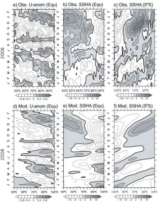
anomalies in August during the onset of the 2006 IOD event are well captured by our model (Figures 3a-b, 3d-e). In the off-equatorial region, our model also reproduces westward propagating positive SSH anomalies during April – August and during the peak phase of the IOD event in October – December (Figures 3c, 3f). However, the model zonal current and SSH anomalies are weaker compared to observations. The weaker amplitude in the model partially is caused by model’s simplified coastline. In addition, the lack of coastal wave dynamics may also contribute to this discrepancy.One of the main advantages of using a linear wave model is the relative important of wind-forced and boundary-generated waves can be diagnosed separately. Figure 4 shows the contributions of wind-forced and boundary generated waves to the zonal current anomalies along the equator during January 2006 through February 2007.
appeared along the equator (Figure 4e) were also mainly influenced by the wind-forced Kelvin waves (Figure 4b), though the reflected Rossby waves (Figure 4c) play dominant role in generating eastward zonal current anomalies near the eastern boundary.
Figure 4 Time-longitude diagrams of model zonal current anomalies along the equator for January 2006 – February 2007, from (a) reflected Kelvin waves, (b) wind-forced Kelvin waves, (c) reflected Rossby waves, (d) wind-forced Rossby waves, and (e) total. The contours in (e) show anomalies of zonal wind stress along the equator. The solid (dotted) lines are for westerly (easterly) anomalies. Contour interval is 2 10-2 N/m2with zero contour highlighted. Note the scale changes in (e).
The role of equatorial oceanic waves in generating SSH anomalies is presented in Figure 5. It is clearly shown that the wind-forced Kelvin waves (Figure 5b) significantly generated negative SSH anomalies at the onset of the IOD in August (Figure 5e). A short reversal of zonal wind anomalies during September (Figure 5e) excited downwelling Kelvin waves (Figure 5b). However, the signals resulted from the wind-forced Kelvin waves are much weaker than the total solution (Figure 5e). We found that wind-forced Rossby waves gave significant contribution in the western basin during this time (Figure 5d).
The model results suggest that the upwelling equatorial waves (negative SSH anomalies) and westward zonal current anomalies that contributed to significant sea surface cooling in the eastern equatorial Indian Ocean during the activation phase of the 2006 IOD event were mainly generated by the wind-forced Kelvin waves.
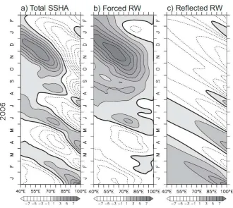
As demonstrated in the previous studies, off-equatorial Rossby waves play an important role in generating SSH and zonal current variability in the western Indian Ocean [15-17]. Here, we focus only on the SSH variations in the off-equatorial region. Figure 6 shows the contribution of wind-forced and boundary generated Rossby waves on the SSH variations along 5S. Our model indicates that elevated sea level in western boundary during the activation of the 2006 IOD event in July – August (Figure 6a) was due to both wind-forced and boundary-generated Rossby waves (Figures 6b,c). The wind-forced downwelling Rossby waves were associated with the easterly wind anomalies along the equator in June (Figure 2a) that caused anomalous surface divergence along the equator east of about 55E (Figures 2c, 3e), and anomalous surface convergence in the off-equatorial region west of about 85E (Figures 2d, 3f). On the other hand, the boundary-generated downwelling Rossby waves were originated from the reflection of downwelling equatorial Kelvin waves that reflected from the eastern boundary in March – April 2006 (2c). Thus, the model suggests that a complex interplay of the wind-forced and boundary-generated downwelling Rossby waves elevated sea level in the western equatorial Indian Ocean during the activation phase of the 2006 IOD event.
4
Discussions
The elevated sea levels in the western equatorial Indian Ocean during the activation phase of the 2006 IOD event was resulted from a complex interplay of the wind-forced and boundary-generated downwelling Rossby waves. The wind-forced downwelling Rossby waves were associated with the easterly winds anomalies along the equator that observed in June (Figure 6b). These anomalous winds caused anomalous surface divergence along the equator east of about 55E and anomalous surface convergence in the off equatorial regions west of about 85E. On the other hand, the boundary-generated downwelling Rossby waves were generated by the eastern-boundary reflection of downwelling equatorial Kelvin waves that arrived in the eastern boundary in March – April 2006 (Figure 6c).
[7] have shown that the cooling tendency in the eastern equatorial Indian Ocean in June 2006 was mainly due to the surface heat flux, since the zonal heat advections were nearly zero at this time. Our model reveals that the boundary-generated Rossby waves originated from upwelling equatorial Kelvin waves forced eastward zonal currents during June [Figure 5c,e]. This may result in a weak contribution of the zonal heat advection on the cooling tendency in the eastern equatorial Indian Ocean in June. In addition, the present of strong anomalous westerly wind anomalies along the equator from late June to early July excited strong downwelling Kelvin waves that warmed the eastern equatorial Indian Ocean and canceled the previous cooling tendency, in agreement with previous studies [18].
5
Conclusion
Role of equatorial oceanic waves in activating the 2006 IOD event is evaluated based on the observations and outputs from a linear wave model. The model is continuously stratified, and the longwave approximation has been use so that only Kelvin and Rossby modes are retained. The model is unbounded in the meridional direction, and it has meridional walls along 40E and 100E. The model is forced by the ECMWF winds from 1980 through 2010.
Our analysis found that anomalous easterly winds along the equator during the activation phase of the 2006 IOD event in August generated upwelling Kelvin waves and westward near-surface zonal currents that contribute to significant sea surface cooling in the eastern equatorial Indian Ocean (Figures 4b, 5b).
Acknowledgment
The author would like to thank Dr. Motoki Nagura for the model output. This study is supported by the Indonesia Toray Science Foundation (ITSF) Research Grant 2012 and by the University of Sriwijaya through Penelitian Unggulan Universitas 2012. This CGCCS contribution number 1201.
References
[1] Saji, N.H., Goswami, B.N., Vinayachandran, P.N. & Yamagata, T., A Dipole Mode in the Tropical Indian Ocean, Nature, 410, pp. 360-363, 1999.
[2] Webster, P.J., Moore, A.W., Loschnigg, J.P. & Leben, R.R., Coupled
Ocean-Atmosphere Dynamics in the Indian Ocean during 1997-98,
[3] Murtugudde, R., McCreary, J.P. & Busalacchi, A.J. Oceanic Processes Associated with Anomalous Events in the Indian Ocean with Relevance to 1997-98, J. Geophys. Res., 105(C2), pp. 3295-3306, 2000.
[4] Saji, N.H., & Yamagata, T. Possible Impacts of Indian Ocean Dipole Mode Events on Global Climate, Clim. Res., 25(2), pp. 151-169, 2003. [5] Horii, T., Hase, H., Ueki, I. & Masumoto, Y.,Oceanic Precondition and
Evolution of the 2006 Indian Ocean Dipole, Geophys. Res. Lett., 35, L03607, doi: 10.1029/2007GL032464, 2008.
[6] Vinayachandran, P.N., Kurian, J. & Neema, C.P.,Indian Ocean Response to Anomalous Conditions in 2006, Geophys. Res. Lett., 34, L15602, doi: 10.1029/2007GL030194, 2007.
[7] Rao, S.A., Luo, J.-J., Behera, S.K. & Yamagata, T., Generation and Termination of Indian Ocean Dipole Events in 2003, 2006 and 2007, Clim. Dyn., 33, pp. 751-767, doi: 10.1007/s00382-008-0498-z, 2009. [8] Cai, W., Pan, A., Roemmich, D., Cowan, T. & Guo, X.,Argo Profiles a
Rare Occurrence of Three Consecutive Positive Indian Ocean Dipole Events, 2006 – 2008, Geophys. Res. Lett., 36, L08701, doi: 10.1029/ 2008GL037038, 2009.
[9] Bonjean, F. & Lagerloef, G.S.E., Diagnostic Model and Analysis of the Surface Currents in the Tropical Pacific Ocean, J. Phys. Oceanogr., 32, pp. 2938-2954, 2002.
[10] Nagura, M. & Mcphaden, M.J., Wyrtki jet Dynamics: Seasonal Variability, J. Geophys. Res., 115, C07009, doi: 10.1029/2009JC005922, 2010a.
[11] Nagura, M. & Mcphaden, M.J., The Dynamics of Zonal Current Variations Associated with the Indian Ocean Dipole, J. Geophys. Res.,
115, C11026, doi: 10.1029/2010JC006423, 2010b.
[12] Clarke, A. J. & Liu, X., Observations and Dynamics of Semiannual and Annual Sea Level near the Eastern Equatorial Indian Ocean Boundary, J. Phys. Oceanogr., 23, pp. 386-399, 1993.
[13] Han, W., Origins and Dynamics of the 90-day and 30-60-day Variations in the Equatorial Indian Ocean, J. Phys. Oceanogr., 35, pp. 708-728, 2005.
[14] Le Blanc, J.L. & Boulanger, J.P., Propagation and Reflection of Long Equatorial Waves in the Indian Ocean from Topex/Poseidon Data during 1993-1998, Climate Dynamics, 17, pp. 547-557, 2001.
[15] Chambers, D.P., Tapley, B.D., Stewart, R.H., Amomalous Warming in the Indian Ocean Coincident with El Niño., J. Geophys. Res.104, pp. 3035-3047, doi: 10.1029/1998JC900085, 1999.
Emphasis on the Indian Ocean Dipole, Deep-Sea Res., 49, pp.1549-1572, 2002.
[17] Feng, M. & Meyers, G., Interannual Variability in the Tropical Indian Ocean: a Two-year Time-scale of Indian Ocean Dipole, Deep-Sea Res.,
50, pp. 2263-2284, 2003.
[18] Horii, T., Masumoto, Y., Ueki, I., Hase, H. & Mizuno, K., Mixed Layer Temperature Balance in the Eastern Indian Ocean during the 2006
Indian Ocean Dipole, J. Geophys. Res., 114, C07011, doi: