ANTARCTIC ICE SHEET SLOPE AND ASPECT BASED ON ICESAT
’
S REPEAT
ORBIT MEASUREMENT
Yuan Lexian a,b, Li Fei a,b,c, *, Zhang Shengkai a,b, *, Xie Surui d
,
Xiao Feng a,b,
Zhu Tingtingb,c, Zhang Yua,ba
Chinese Antarctic Center of Surveying and Mapping, Wuhan University, Wuhan, 430079, China b
Collaborative Innovation Center for Territorial Sovereignty and Maritime Rights,Wuhan University, Wuhan, 430079, China c
State Key Laboratory of Information Engineering in Surveying, Mapping and Remote Sensing, Wuhan University, Wuhan, 430079, China
d
School of Geosciences, University of South Florida, Tampa, FL, 33601, USA
KEY WORDS: slope, aspect, Antarctic ice sheet, ICESat, repeat orbit
ABSTRACT:
Accurate information of ice sheet surface slope is essential for estimating elevation change by satellite altimetry measurement. A study is carried out to recover surface slope of Antarctic ice sheet from Ice, Cloud and land Elevation Satellite (ICESat) elevation measurements based on repeat orbits. ICESat provides repeat ground tracks within 200 meters in cross-track direction and 170 meters in along-track direction for most areas of Antarctic ice sheet. Both cross-track and along-track surface slopes could be obtained by adjacent repeat ground tracks. Combining those measurements yields a surface slope model with resolution of approximately 200 meters. An algorithm considering elevation change is developed to estimate the surface slope of Antarctic ice sheet. Three Antarctic Digital Elevation Models (DEMs) were used to calculate surface slopes. The surface slopes from DEMs are compared with estimates by using in situ GPS data in Dome A, the summit of Antarctic ice sheet. Our results reveal an average surface slope difference of 0.02 degree in Dome A. High resolution remote sensing images are also used in comparing the results derived from other DEMs and this paper. The comparison implies that our results have a slightly better coherence with GPS observation than results from DEMs, but our results provide more details and perform higher accuracy in coastal areas because of the higher resolution for ICESat measurements. Ice divides are estimated based on the aspect, and are weakly consistent with ice divides from other method in coastal regions.
1. INTRODUCTION
Slope and aspect of Antarctic ice sheet are important parameters for Antarctic drainage divides, glacier movement, morphometric measurements, and many other studies. The ice velocity increases in the area with steep slope (Zhang et al., 2008). Slope and aspect are usually the secondary products of Digital Elevation Models (DEMs). Different algorithms for calculating slope and aspect are proposed (Travis et al., 1975; Evans, 1980; Horn, 1981), the difference between most algorithms that compute slope and aspect is the number of grid cell values used and weights given to each of these cell values (Kevin, 1998). Although different algorithms produce different results, the most significant outcome is that slope varies inversely with different resolutions (Zhang et al., 1999).
The spatial resolution of Antarctic DEM is limited by poor survey data because of the harsh ice environment. Bamber et al. (2009) assessed the optimum resolution for Antarctic DEM to be 1 km by combining satellite radar and laser data and developed a DEM of Antarctica. National Snow and Ice Data Center (NSIDC) developed a DEM of Antarctica with resolution of 500 meters using laser altimeter measurements from Ice, Cloud and land Elevation Satellite (ICESat) (DiMarzio et al., 2007). Although one of the frequently used Antarctic DEMs which was created by the Radarsat Antarctic Mapping Project (RAMP) has horizontal resolution of 200 meters over rugged mountains (Liu et al., 1999), for most areas
of the Antarctic ice sheet, a true spatial resolution of higher than 500 meters is unavailable. Estimating high resolution slope values in Antarctic ice sheet seems to be difficult.
The ICESat is the first polar orbiting satellite to carry a laser altimeter on earth (Schutz et al., 2005). The slope and aspect with higher resolution can be determined using ICESat data because ICESat ground tracks don’t repeat exactly and the mean distance between different ICESat ground repeat tracks is about 200 meters. Yi et al. (2005) calculated the slope of Greenland ice sheet by ICESat’s 8-day repeat orbit. ICESat also provide 91-day repeat orbit with much denser coverage than 8-day repeat orbit, but the elevation changes of the ice sheet must be considered when using 91-day repeat orbit data (Li et al., 2016). In this paper, slope and aspect of Antarctic ice sheet with resolution of about 200 m are calculated using the 91-day repeat orbit data of ICESat. The surface elevation changes of the ice sheet are also considered in our calculation.
2. DATA
ICESat was launched by NASA into a 600 km altitude orbit with a 94 degree inclination. Geoscience Laser Altimeter System (GLAS) on-board ICESat collected data from February 20th, 2003 to October 11th, 2009. There are 3 lasers named Laser 1, 2 and 3 mounted on GLAS, with one laser operating a time. ICESat has an 8-day repeat orbit during the operation time of Laser 1 and early time of Laser 2 until October 4th, 2003, and
The International Archives of the Photogrammetry, Remote Sensing and Spatial Information Sciences, Volume XLII-2/W7, 2017 ISPRS Geospatial Week 2017, 18–22 September 2017, Wuhan, China
a 91-day repeat orbit has been used in the following ICESat operation time (Schutz et al., 2005). The 91-day repeat orbit data are used in this paper because of the denser coverage. The diameter of ICESat footpoint is about 70 meters and is separated 172 meters apart along track on the ground.
The level 2 Antarctic Ice Sheet Altimetry Data product (GLA12) are used to calculate slope and aspect in this study. The following parameters are obtained to evaluate the quality of the shots: elevation use flag, orbit flag and attitude flag. We exclude all shots with poor quality. Shots with gain more than 100 are also rejected, and only those shots with energy <13.1fJ when the gain between 14 and 100 are used (Nguyen and Herring, 2005). Saturation correction is also applied to the elevations. The locations of GLA12 data are converted from TOPEX/Poseidon to WGS-84 ellipsoid for consistency with GPS data. The remaining ICESat ground data are showed in Fig. 1 after filtering and corrections.
Figure 1. ICESat ground tracks on Antarctic ice sheet after filtering and corrections
3. ALGORITHM
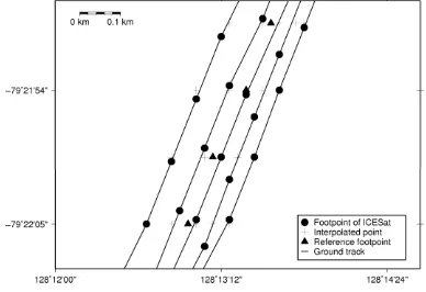
We use along track interpolation to adjust the footpoints to the same latitude as shown by crosses in figure 2. Elevations of the crosses are extracted by linear interpolation between the two
Figure 2. ICESat ground tracks and reference track
Surface elevations of Antarctic ice sheet are easily affected by climate change. Since the data for different repeat tracks are collected in different times, elevation changes of the ice sheet must be considered when compute slopes by repeat tracks. Both annual and inter-annual impacts for the elevation changes of Antarctic ice sheet have been considered when estimating the slopes in East-West direction. The following equation is used in this paper:
parameters to be solved. Fewer observations will lead to lower precision. To reduce error, we only estimate parameters when there are more than 2 redundant observations. We get the following formula by expending the equation (1):
i
parameters are calculated using least square method.
The elevation of the reference point
h
0 is used to estimate theslope in along-track direction. Intersection angle between East-West direction and along-track direction is calculated using inverse solution of geodetic problem. Slope and aspect can be determined by combining slopes in East-West direction and along-track direction.
4. RESULTS AND ANALYSIS
4.1 SLOPE
The Antarctic ice sheet surface slope map from ICESat repeat-track data is shown in Figure 3. The results cannot cover the whole Antarctic ice sheet because the resolution is 200 meters. Slopes at the areas between different repeat-tracks are invalid. The surface slopes for most of Antarctic ice sheet areas are <0.5 degree. In the coastal margins and mountain areas such as Transantarctic Mountains and Antarctic Peninsula, the slopes can be up to >1 degree. The surface slopes of Antarcitc ice sheet also reveal some subtle features, such as ice divides and Lake Vostok, where the slopes are mostly <0.1 degree.
Gaps of the derived slope map are mainly due to the coverage and quality of the data. Slope calculated by the repeat tracks in this paper performs well near the satellite tracks, but the method may not be appropriate for the areas far away from the tracks, which results in the blank gaps between different tracks in figure 3. According to equation (2), the slope can be calculated when there are data from at least 7 different periods, but some of GLA12 data are removed because of the poor qualities due to the complex surface terrain, clouds and other factors, so there are more data gaps in West Antarctic areas.
Figure 3. Antarctic ice sheet surface slope from ICESat repeat orbit data.
GPS measurements and satellite images are used to estimate the accuracy of the slope from this study. The slopes of the ice sheet calculated by elevations from dense GPS data are compared with slopes from repeat-track method and other DEMs. Satellite images can also provide a sketch of slopes. Comparison with hillshade from high resolution satellite images should reveal the relative accuracy of slopes from different DEMs.
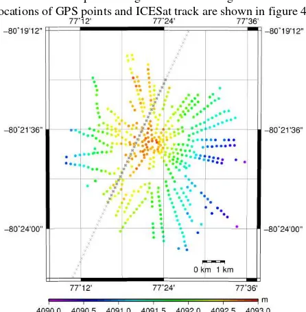
The surface topography of Dome A was measured by real-time kinematic GPS using two Leica SR530 dual-frequency GPS receivers during the 21st Chinese National Antarctic Research Expedition (CHINARE) in January, 2005, which covers an area of ~60 km2 at a spatial resolution of about 200 meters (Zhang et al., 2007). GPS data were processed by using GAMIT/GLOBK software. More than 400 GPS points with errors smaller than 0.10 meters in vertical direction were used in this study. One of the ICESat tracks pass through the GPS data region. The locations of GPS points and ICESat track are shown in figure 4.
Figure 4. GPS data and ICESat track in Dome A
Slopes for the grey footpoints of ICESat track in figure 4 are estimated using GPS data, three DEMs mentioned above and repeat-track method respectively. Differences between slopes obtained from GPS data and other methods are calculated. The statistics presented in table 1 are mean difference and standard deviation around the mean difference.
The largest standard deviation of slope difference is between GPS and RAMP DEM. There are similar mean differences and standard deviations for slopes derived from Bamber DEM and ICESat DEM.
The mean difference for repeat-track method is slightly smaller than Bamber DEM and ICESat DEM results. Since the terrain in Dome A area is quite flat and the hypsographic feature is simple, the differences between this study and those two DEMs are insignificant.
Slopes derived from Bamber DEM and ICESat DEM have comparable accuracy while slopes derived from repeat-track method are slightly better in the region with simple surface feature such as Dome A area.
Method
Mean difference
(degree)
Standard deviation (degree)
GPS-Bamber DEM 0.03 0.02
GPS-ICESat DEM 0.03 0.02
GPS-RAMP DEM 0.02 0.05
GPS-Repeat-track 0.02 0.02
Table 1.Comparison between the slopes derived from GPS data and other methods
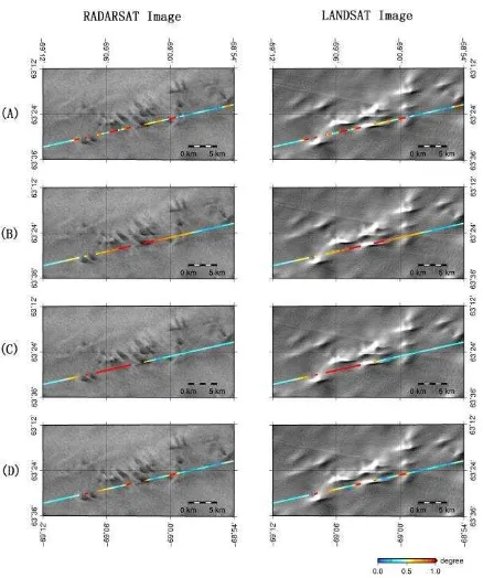
Remote sensing image data are used to validate the reliability of the slope in this study since GPS data are only available in limited areas in Antarctica. Radar image from RADARSAT-1 acquired in 1997 with resolution of 100 meters and optical image obtained in 2016 from LANDSAT-8 with resolution of 30 meters are used.
The images locate in the west of Amery ice shelf named Mac. Robertson Land with complex terrain surface features. Although there are 19 years difference between the two different images, the topographic features on RADARSAT-1 and LANDSAT images are still similar. There are a few elevation changes in this area and the elevation changes were supposed to be identical in a small area (Gunter et al., 2009). The differences of the two images may come from the different reflection characters for radar image and the optical image. We assume that the slopes in flat regions are small, while large in mountainous regions. Regions with large slopes should have more shadows on satellite images.
Slopes of ICESat track deserved from different methods and DEMs are also shown in figure 5. The slopes derived from this paper (A) show great agreement with the images, and much more details had been showed for the slopes derived from this paper compared with other DEMs. Smooth slope values in Bamber DEM results and RAMP DEM results in figure (B) and (C) are due to the resolution and interpolation. The resolutions for Bamber DEM and RAMP DEM are both lower than 200 meters, while the distance for adjacent ICESat surface footprints are only 170 meters, most of the slopes are calculated by interpolation.
Slopes estimated by ICESat repeat tracks perform better than slopes derived from lower resolution DEMs in mountainous regions. More detailed terrain slope information can be derived from the slopes calculated in this paper.
Figure 5. LANDSAT image and slopes of ICESat track derived from repeat-track method (A), RAMP DEM (B), Bamber DEM
(C) and ICESat DEM (D).
4.2 ASPECT
The aspect distributions of Antarctic ice sheet are also calculated in this paper, which is shown in figure 6. From dome areas to ice shelf, the tendencies of the aspects are almost the same overall. Different aspects appear at different sides of the three biggest ice shelfs in Antarctic (Ross Ice Shelf, Ronne Ice Shelf and Amery Ice Shelf).
Since ice stream directions are determined by the aspect of the terrain surface. Most of the ice divides located in the places where the aspect changes the directions. Based on this principle, ice divides are delineated by the aspect in this paper. Ice divides cannot be delineated to more detailed in West Antarctica due to the insufficiency of the data.
Comparison of the ice divides defined by this paper, Rignot et al., (2008) and Zwally et al., (2012) are shown in figure 7. The agreement is good in the inland ice sheet with high elevations. However, the aggregation of basins into sectors differs in some instances especially at the coastal regions.
The divides are obvious in inland ice sheet because of the simple topography features. However, the terrain features are more complex in coastal areas, and the aspect we estimate has resolution about 200 meters, which would confuse the features of the ice divides. The ambiguous boundary between different aspects led to the inconsistency of ice divides in some regions.
Figure 6. Aspect distributions and drainage basins of Antarctic ice sheet.
Figure 7. Comparison of the ice divides of this paper (red borders) and Zwally et al., 2012 (blue borders) and Rignot et al.,
(2008) (dark green borders).
5. CONCLUTION
A method to estimate the slope and aspect of Antarctic Ice Sheet with about 200 meters resolution based on ICESat repeat-track is proposed. The elevation change is considered in the calculation. Slopes and aspects of the Antarctic Ice Sheet are calculated by using this method. Slopes estimated in this paper are compared with slopes derived from three other DEMs in two different areas (Dome A and a mountainous area near the coast). The accuracy of the slopes calculated in this paper is slightly better in flat areas by comparing the results with in situ GPS data, while the accuracy is much higher in the region with complex surface feature by comparing with high resolution
remote sensing images. Although the ice divides are determined by the aspect calculated in this paper, there are some limitations in delineating ice divides.
ACKNOWLEDGEMENTS
This study is supported by the State Key Program of National Natural Science of China, No. 41531069, the National Key R&D Program of China, No. 2017YFA0603102, the Independent research project of Wuhan University, 2017, No. 2042017kf0209, the National Natural Science Foundation of China, No. 41176173 and 41476163, the Polar Environment Comprehensive Investigation and Assessment Programs of China, No. CHINARE2017, the China Postdoctoral Science Foundation, No. 2017M612507.
REFERENCES
Bamber J. L., Gomez-Dans J. L., Griggs J. A., 2009. A new 1 km digital elevation model of the Antarctic derived from combined satellite radar and laser data. Part 1: data and methods. The Cryosphere, 3, pp. 101–111.
DiMarzio J., Brenner A., Schutz R., et al., 2007. GLAS/ICESat 500 m laser altimetry digital elevation model of Antarctica. Boulder, Colorado USA: National Snow and Ice Data Center. Evans I. S., 1980. An integrated system of terrain analysis and slope mapping. Z. Geomorphol. Supp., 36, pp. 274-295. Gunter Brian, T. Urban, R. Riva, et al., 2009. A comparison of coincident GRACE and ICESat data over Antarctica. J Geodesy, 83(11), pp. 1051-1060.
Horn B. K. P., 1981. Hill shading and reflectance map. Proceedings of the IEEE, 69(1), pp. 14±47.
Li Fei, Yuan Lexian, Zhang Shengkai, et al., 2016. Mass change of the Antarctic Ice Sheet derived from ICESat laser altimetry. Chinese J. Geophys., 59(1), pp. 93-100.
Liu H., Jezek K. C., Li B., 1999. Development of an Antarctic digital elevation model by integrating cartographic and remotely sensed data: a geographic information system based approach. Journal of Geophysical Research: Solid Earth, 104(B10), pp. 199-213.
Kevin H. Jones, 1998. A COMPARISON OF ALGORITHMS USED TO COMPUTE HILL SLOPE AS A PROPERTY OF THE DEM. Computers & Geosciences, 24(4), pp. 315-323. Rignot Eric, Jonathan L. Bamber, Michiel R. van den Broeke, et al., 2008. Recent Antarctic ice mass loss from radar interferometry and regional climate modelling. Nature Geoscience 1, pp. 106–110.
Schutz B. E., Zwally H. J., Shuman C. A., et al., 2005. Overview of the ICESat mission. Geophys Res Lett, 32(21), L21S01.
Nguyen A. T., Herring T. A., 2005. Analysis of ICESat data using Kalman filter and kriging to study height changes in East Antarctica . Geophys Res Lett, 32(23), L23S03.
Travis M. R., Elsner, G. H., Iverson, W. D. et al., 1975. VIEWIT computation of seen areas, slope and aspect for land-use planning. US Department of Agriculture Forest Service Gen. Techn. PSW 11/1975, Pacific Southwest Forest and Range Experimental Station, Berkley, California, USA.
Yi Donghui, Zwally H. Jay, Sun Xiaoli, 2005. ICESat measurement of Greenland ice sheet surface slope and roughness. Annals of Glaciology, 42(1), pp. 83-89.
Zwally, H. Jay, Mario B. Giovinetto, Matthew A. Beckley, et al., 2012, Antarctic and Greenland Drainage Systems, GSFC
Cryospheric Sciences Laboratory, at
http://icesat4.gsfc.nasa.gov/cryo_data/ant_grn_drainage_system s.php.
Zhang Shengkai, E Dongchen, Wang Zemin, et al, 2007. Surface topography around the summit of Dome A, Antarctic, from real-time kinematic GPS. Journal of Glaciology. 53, pp. 159-160.
Zhang Shengkai, E Dongchen, Wang Zemin, et al., 2008. Ice velocity from static GPS observations along the transect from Zhongshan station to Dome A, East Antarctica. Annals of Glaciology, 48, pp. 113-118.
Zhang Xiaoyang, Nick A. Drake, John Wainwright, et al., 1999. COMPARISON OF SLOPE ESTIMATES FROM LOW RESOLUTION DEMS: SCALING ISSUES AND A FRACTAL METHOD FOR THEIR SOLUTION. Earth Surface Processes and Landforms, 24, pp. 763-779.