TREND ANALYSIS OF SOIL SALINITY IN DIFFERENT LAND COVER TYPES USING
LANDSAT TIME SERIES DATA (CASE STUDY BAKHTEGAN SALT LAKE)
Mohammad Mahdi Taghadosi a, Mahdi Hasanlou a*
a School of Surveying and Geospatial Engineering, College of Engineering, University of Tehran, Tehran, Iran (mahdi.taghadosi, hasanlou)@ut.ac.ir
KEYWORDS: Soil Salinity, Per-pixel Trend Analysis, Land Covers, Salinity Indicators, Slope Index, Landsat Time Series Data
ABSTRACT:
Soil salinity is one of the main causes of desertification and land degradation which has negative impacts on soil fertility and crop productivity. Monitoring salt affected areas and assessing land cover changes, which caused by salinization, can be an effective approach to rehabilitate saline soils and prevent further salinization of agricultural fields. Using potential of satellite imagery taken over time along with remote sensing techniques, makes it possible to determine salinity changes at regional scales. This study deals with monitoring salinity changes and trend of the expansion in different land cover types of Bakhtegan Salt Lake district during the last two decades using multi-temporal Landsat images. For this purpose, per-pixel trend analysis of soil salinity during years 2000 to 2016 was performed and slope index maps of the best salinity indicators were generated for each pixel in the scene. The results of this study revealed that vegetation indices (GDVI and EVI)and also salinity indices (SI-1 and SI-3) have great potential to assess soil salinity trends in vegetation and bare soil lands respectively due to more sensitivity to salt features over years of study. In addition, images of May had the best performance to highlight changes in pixels among different months of the year. A comparative analysis of different slope index maps shows that more than 76% of vegetated areas have experienced negative trends during 17 years, of which about 34% are moderately and highly saline. This percent is increased to 92% for bare soil lands and 29% of salt affected soils had severe salinization. It can be concluded that the areas, which are close to the lake, are more affected by salinity and salts from the lake were brought into the soil which will lead to loss of soil productivity ultimately.
1. INTRODUCTION
Salinization is one of the serious environmental hazards and the major factor that causes land degradation and desertification (Allbed et al., 2014a; Allbed and Kumar, 2013; Metternicht and Zinck, 2003a). It can occur through natural processes such as physical and chemical weathering, evapotranspiration, drought and lack of precipitation, or caused by human activities such as using salt-rich irrigation, inefficient water use, poor drainage, construction of dam, etc., which leads to reduced soil fertility and loss of crop productivity ultimately (“Soil salinization,”2017). Detecting salt-affected areas and determining the extent of changes can be an effective approach in monitoring soil salinity and its impact on land management (Allbed and Kumar, 2013; Metternicht and Zinck, 2008). Using multispectral satellite images taken over time along with remote sensing techniques, make it possible to evaluate changes in salt-affected lands through multi-temporal analysis. Saline soils can be detected directly from multispectral image bands through high spectral reflectance in the visible and near-infrared (NIR) range of the electromagnetic spectrum on bare soils or indirectly from changes in crop condition and loss of agricultural productivity in farmlands (Allbed and Kumar, 2013; Metternicht and Zinck, 2003a). Both direct and indirect methods should be considered for assessing soil salinity changes, especially in large-scale areas, which consist of different land cover types.
In recent years, various salinity and vegetation indices have been developed to detect salt affected areas and monitoring soil salinity (Allbed et al., 2014a; Allbed and Kumar, 2013; Gorji et al., 2017; Ivushkin et al., 2017; Satir and Berberoglu, 2016). Vegetation indices are commonly used to highlight vegetated areas from spectral behaviours of vegetation (Allbed and Kumar, 2013; Ji-hua et al., 2008). Due to the expansion of salinity in affected areas and its adverse effects on plant growth, a decrease
* Corresponding author
in vegetation index values can be interpreted as soil degradation and salinity spread(Allbed et al., 2014b; Dubovyk et al., 2013; Metternicht and Zinck, 2003b). In contrast, salinity indices highlight spectral reflectance values of salt affected regions in the case of less vegetation, therefore, increase in salinity index values during years of study represents salinization of bare soil lands. Previous studies have shown the potential of using direct and indirect salinity indicators to detect salt affected areas and assessing salinity changes. Ji-hua et al. assessed different methods to monitor large-scale crop condition using satellite images. Different monitoring method was evaluated and vegetation indices were used to monitor crop condition. The results of this study revealed that more and more indices should be used to monitor crop condition in order to increase the monitoring precision (Ji-hua et al., 2008). Dubovyk et al. used time series of the 250m MODIS NDVI over growing seasons of 2000-2010 in the Khorezm region, Uzbekistan, to assess negative vegetation trend which was interpreted as an indicator of land degradation(Dubovyk et al., 2013). Allbed et al. assessed soil salinity levels in the eastern province of Saudi Arabia, which is dominated by date palm vegetation, using IKONOS satellite images. Thirteen vegetation and salinity indices were extracted from IKONOS satellite images and predictive power of these indices for soil salinity was examined. Among these indices, the SAVI, NDSI, and SI-T had the best precision to assess soil salinity in vegetated lands and also, the NDSI and SI-T showed the highest correlation for bare soils (Allbed et al., 2014b). Imanyfar et al. determined the spatial pattern of Oak decline in Ilam province of Iran using Landsat time series data between years 2000 and 2015. In this study, the slope of temporal variation of five appropriate vegetation indices was extracted and the Oak forests were classified into four categories according to the severity of Oak decline. The results of this study showed that
the EVI index had the best performance between selected vegetation indices (Imanyfar and Hasanlou, 2017). Gorji et al. assessed soil salinity changes in the vicinity of Tuz Salt Lake region in Turkey using multi-temporal Landsat-5 and Landsat-8 images obtained between 1990 and 2015. Using 28 soil samples and also five soil salinity indices which obtained from satellite images, linear and exponential regression analysis were performed and salinity maps were generated for years of study. The results of this study indicated thatland cover changes in the study area from years 2000 to 2006, and from 2006 to 2012. The results also revealed that salinity index (SI) had the best performance to detect salt affected areas from satellite images according to the results of linear and exponential regression analysis(Gorji et al., 2017). Due to the fact that the study area consists of different land cover types such as vegetation and bare soil lands, this paper aims to assess the effects of salinity on both vegetation and bare soil lands using Landsat time series data during the last two decades.
2. MATERIALS AND METHODS 2.1 Study Area
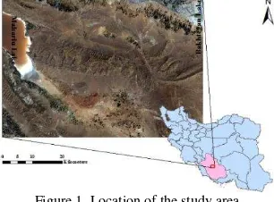
Bakhtegan Salt Lake is Iran’s second largest lake (Figure1), with a surface area of 3500 square kilometers, located in Fars Province, southern Iran, about 160km east of Shiraz and 15km west of the town (“Bakhtegan Lake - Wikipedia,” 2017). This region has suffered from salinization during the last two decades due to the lack of adequate rainfall and construction of the several dams on the Kor river which flowed into the lake. The dams on the Kor river had significantly reduced water flow into the lake, leading to widespread salinization. For the purpose of assessing salinity effect on both vegetation and bare soil lands the area (29°8’27’’N to 29°34’28’’N, 52°47’5’’E to 53°28’30’’), around the lake were selected. This area, which located west of the Bakhtegan Lake, is composed of three land cover classes including (1) water lake, (2) soil, and (3) vegetation and affected by salinity due to its vicinity to the Salt Lake.
Figure 1. Location of the study area
2.2 Remotely sensed data
Landsat imageries have a great potential to assess salinity changes due to their large time series database, relatively good spatial resolution (30m30m) and providing spectral bands in visible and near-infrared (NIR) range of the electromagnetic spectrum. This study considers seventeen years of Landsat 7 and 8 data. Firstly, monthly Landsat 8 images from April 2013 to December 2016 were obtained to be used in four years analysis of salinity changes. Then Landsat 7 images of late May from 2000 to 2013 were acquired for trend analysis of soil salinity during seventeen years. This time had the best performance to evaluate changes according to the results of the four years study. 2.3 Utilized methodology
According to the results of the previous studies, monitoring soil salinity and assessing changes in salt affected areas can be performed through different salinity/vegetation indices using Landsat imagery. Vegetation indices can be applied to Landsat time series data in the areas covered by vegetation to evaluate the reduction in plant growth and yield loss during the time period. Salinity indices are also used to assess spectral reflectance of salt
affected soils in bare lands by measuring indices values and rate of changes during seventeen years study. Due to the presence of two major types of land cover in the study area and the opposite behaviors of salinity and vegetation indices in groundvegetation and bare soil lands, the distinction between the two land cover types should be firstly considered. Thus, supervised maximum likelihood classification algorithm which represents the best relative performance against other classification approaches was performed to separate land cover classes of the whole scene to (1) water body, (2) bare soil, and (3) vegetation. Soil and vegetation mask was then generated based on the results of the classification. Vegetation indices which indicate amounts of vegetation should be applied to vegetation pixels and salinity indices which represent the high spectral reflectance of saline soils should be applied to bare soil lands pixels.
Among the large number of vegetation and salinity indices that have been developed for salinity detection in recent years, four vegetation indices NDVI, EVI, SAVI, and GDVI and four salinity indices SI-1, SI-2, SI-3, and BI, which had the best performance based on the results of the previous papers, were selected (Table 1). From selected indices, the following criteria were used to choose the best salinity indicators in the study area: (a) correlation coefficient, (b) mean of standard deviation, and (c) trend line slope of the mean index. In the next step, evaluating the variation of salinity indicators in different months of the year from January to December should be carried out to select the best time for trend analysis of soil salinity. To this purpose, four years analysis of monthly changes from April 2013 to December 2016 was performed using Landsat 8 images. The month which has the most increase in salinity indices values in bare soils and the most reduction in vegetation indices values in vegetation lands is considered the optimal time to assess changes due to more sensitivity to salt features of two land cover types over years. In this regard, images of late May were selected. Finally, slope map of optimal VI/SI indices of May images during 2000 to 2016 is created using Landsat7, 8 data to assess the rate of change for each pixel through salinity indicators. The slopes with greater absolute values, indicate large amounts of changes in both land cover pixels due to salinity occurrence and correspond to highly salt affected soils over the years of study. The areas with fewer slope values represent unchanged pixels and correspond to normal or slightly affected soils. According to this, the study area was divided into different degrees of salinity which are: (1) non-saline, (2) slightly non-saline, (3) moderately non-saline, and (4) highly saline. In addition to thresholding, K-means clustering method is also applied to segment the slope image map of both land cover types to different salinity classes. The results of obtained salinity classes of both methods were compared with each other to assess the effectiveness of used methods and the extent of salinity hazard in the study area during the last two decades.
Figure 2. Flowchart of proposed method for trend analysis of soil salinity and mapping salinity changes.
3. RESULTS AND DISCUSSION 3.1 Pre-processing of Landsat data
Pre-processing of remotely sensed data is often necessary to prepare data for further usage. Due to a comparative analysis of Landsat time series data which were acquired in different years and also per-pixel temporal trend analysis of soil salinity in this study, pre-processing of Landsat 7 and 8 images is mandatory to ensure meaningful analysis and results. Several pre-processing steps should be considered for all images in order to eliminate or reduce radiometric and geometric distortions of data which include (1) mask out cloud pixels, (2) radiometric calibration to reduce digital numbers errors and convert it to Top of Atmosphere (TOA) reflectance, and (3) atmospheric correction to remove the effect of atmosphere on the reflectance values. In addition, because of the failure of the scan line corrector of Landsat 7 data after May 31, 2003, a number of methods have been developed to fill the gaps. Among the proposed methods, local linear histogram matching (LLHM) technique which provides more accurate results and greater precision was chosen according to (Scaramuzza et al., 2004).
Since the assessment of salinization in the study area is based on changes in individual pixel values and calculating the slope index for each pixel during seventeen years of study, image co-registration should be performed to align Landsat time series data geometrically so that corresponding pixels represents the same area in the scene and become comparable during the time period 2000 to 2016.
3.2 Classification and generation of land masks
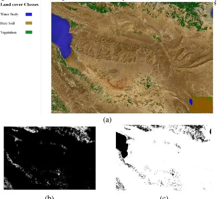
Regarding the aim of the study to assess the effects of salinization in both land covers, the distinction of vegetation and bare soil pixels was performed to be analyzed separately. Using supervised maximum likelihood classification algorithm which provides better accuracy, the study area was divided into three classes: (1) water body, (2) bare soil, and (3) vegetation as shown in Figure 3(a). Vegetation mask which only represents vegetation pixels in the scene was then generated to be used in the analysis of salt affected areas in vegetation lands using results of the classification. The same approach was considered to build soil mask in the areas covered by bare soils based on classification results. Figure 3 (b), Figure 3 (c) show the built mask of vegetation and soil pixels in the study area.
(a)
(b) (c)
Figure 3. The distinction of different land cover types pixels based on the results of the classification: (a) maximum likelihood classification results with three classes, (b) vegetation mask pixels (black: veg., white: veg.), and (c) soil mask pixels (black:
non-soil, white: soil).
3.3 Selection of optimal VI/SI indices
Selecting the best salinity indicators which properly characterize salinization in the study area is needed. Four vegetation indices which are considered as indirect salinity indicators were chosen based on the relatively good performance for detecting soil salinity in the previous papers (Allbed and Kumar, 2013; Satir and Berberoglu, 2016; Wu et al., 2014). These indices were then applied to vegetation pixels and two of them which had the most sensitivity to plant loss were selected according to decision criteria. For bare soil pixels, the same approach was done and four salinity indices which count as direct salinity indicator were firstly selected based on (Allbed and Kumar, 2013; Azabdaftari and Sunar, 2016; Elhag, 2016; Gorji et al., 2017). Then evaluation of these salinity indices is done to select the two best direct salinity indicators. Table 1 shows primarily selected salinity indicators in the direct and indirect way.
Table 1. Direct and indirect salinity indicators for detecting and assessing salt affected areas
Vegetation Indices Salinity Indices
NDVI NIR − R
NIR + R SI-1 √ Green2+ Red2+ NIR2
EVI . NIR − Red
NIR + ∗ Red − . ∗ Blue + SI-2 Red × NIRGreen
SAVI + L NIR − Red
NIR + Red + L SI-3 √Green × Red
GDVI NIR
n− Rn
NIRn+ Rn, n = BI √ Red2+ NIR2
Among eight popular salinity indicators which were selected to assess changes, some of them have more sensitivity to salt features and provide better accuracy in our study area. Indices should be applied to corresponding land cover classes using built masks to evaluate efficiency. For this purpose, following criteria were used and eight selected indices were compared to determine the best salinity indices in bare soils and the best vegetation indices in vegetated lands.
3.3.1 Correlation coefficient
This criterion can be used to measure the correlation between indicators. In the case of vegetation assessment, GDVI and EVI had the most correlation coefficient of 0.991 which indicate a strong relationship between these two indirect salinity indicators. In bare soil pixels, SI-1 and SI-3 were the best with correlation 0.972. Regarding this criteria, EVI and GDVI as indirect salinity indicators in vegetated lands and SI-1 and SI-3 as direct salinity indicator in bare soil lands were selected.
3.3.2 Mean of standard deviation
This criterion indicates the amounts that indices values are close to the mean. Since it needs to highlight changes in indices values which relate to salinity, greater values of standard deviations should be considered which means that pixel values spread out over a wider range of values and change more. Mean of the standard deviation of indiceswas then calculated. In vegetated lands, GDVI and NDVI with values of 0.112 and 0.083 had greater standard deviation. In bare soil lands, SI-2 and SI-3 with a standard deviation of 0.056 and 0.037 had greater values than others. Thus, mentioned salinity indicators were selected according to this criteria.
3.3.3 Trend line slope of mean index
Drawing trend line from mean values of indicators, which represents general behaviors of salinity in the scene, can be used to determine the rate of changes over time. It should be noted that mean values have to be calculated from images of particular time so that it can be comparable during years of study (e.g. images of May during four years). Trend line slopes were then calculated to assess the rate of changes in mean values during years 2013 to
2016. In the case of vegetation, reduction of mean values would be expected as a result of plant loss. Thus, trend line slopes are negative and high absolute values of slopes correspond to more changes. From four mentioned indices GDVI and NDVI with -0.009 and -0.0006 slope values had the most change during four years. In bare soil lands, due to increase in spectral reflectance which caused by salinization, mean salinity indices tend to increase over time. Thus trend line slopes are positive and those which had the most increase in bare soil lands were selected. From mentioned salinity indices SI-1 and SI-3 with 0.0006 and 0.00001 slope values were chosen.
According to the results of the three mentioned criteria, GDVI had the best performance in case of vegetated lands. EVI and NDVI had also relatively good performance, but due to the similar formula of GDVI and NDVI, we decided to use EVI index to assess changes differently. In the case of bare soil lands and salinity indices, SI-1 and SI-3 had the best performance in four years analysis so that they were selected to be used in trend analysis of soil salinity during 2000 to 2016.
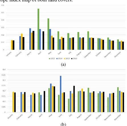
3.4 Determining the best time to assess salinity changes Regarding the accessibility to Landsat time series data and also providing images every 16 days for each location on Earth, it is possible to monitor soil salinity and assess the rate of changes at different times of the year and various time intervals. However, selecting the best time of the year to perform trend analysis and evaluate changes which properly represents the most variation in pixels is necessary. Accordingly, as mentioned above, four years analysis of monthly changes was firstly performed using Landsat 8 images during April 2013 to December 2016. Mean values of both indicators were calculated from Landsat 8 images in every month. Comparative assessment of mean values for each month was then performed in both land covers during four years. It can be expected that in vegetated lands mean values are going to decrease due to plant loss. According to this, the best time can be detected from the month which has the most decrease in mean values which means that in this time vegetation pixels represent the most sensitivity to salinization. Figure 4 (a) illustrates the mean values of EVI index during four years. As it is seen, reduction of mean values is observed in every month. This change is highlighted in images of April and May (Images of January 2014 and April 2015 were excluded due to cloud-cover). In bare soil land pixels, we expect to see the increase in mean values due to the increment of spectral reflectance of salt affected bare soils. Figure 4 (b) indicate the relative increase of mean values in the SI-1 index over time as expected. Images of May and June represent more increase in values during the time. However, these changes are less than the changes were observed in vegetation indices. We also examined GDVI and SI-3 Indices, which were selected in previous step (3.3), and the results were the same. Finally, images of May were chosen due to more sensitivity to salt features in both land cover types according to the results of the four years analysis.
3.5 Applying optimal salinity indicators to Landsat time series data
Regarding the optimal time for trend analysis of soil salinity (3.4) and also the best salinity indicators which were acquired from (3.3), assessing salinity changes can be performed in different land covers during seventeen years using Landsat 7 (2000 -2013) and Landsat 8 (2-13 -2016) images. To evaluate the rate of changes and calculate slope index for each pixel in the scene, image co-registration was performed to seventeen years data based on (3.1). Then, GDVI and EVI were applied to vegetation pixels and SI-1 and SI-3 were applied to bare soil pixels. In the
next step, the best-fit line will be drawn for each pixel to generate slope index map of both land covers.
(a)
(b)
Figure 4. Mean changes of optimal salinity indicators during four years: (a) EVI vegetation index and (b) SI-1 salinity index
3.6 Fitting the best line to corresponding pixels and generate slope index map
As a result of image co-registration process, corresponding pixels represent the same area in the scene, therefore, a trend line can be drawn for each pixel through 17 points and slope map of each indicator will be created using trend line slopes. These slopes indicate the rate of changes in pixel index values and correspond to land cover variations of both vegetation and bare soil lands which caused by salinity. In both cases, the slopes with greater absolute values, indicate large amounts of changes in pixels and correspond to highly salt-affected lands. In contrast, pixels with fewer slope values do not change significantly and are considered as normal or slightly affected soils over years. To determine general behaviors of pixel slopes in the scene mean and standard deviation of created slope maps was calculated as shown in Table 2.
Table 2. Mean and Standard deviation of generated slope maps from optimal indicators
Slope Index Statistics Mean Standard Deviation
EVI -0.0016 0.0084
GDVI -0.0075 0.0125
SI-1 0.0028 0.0021
SI-3 0.0053 0.0039
3.7 Mapping salinity changes
Slope maps of the study area which were generated in the previous step were assessed to obtain map of salinity changes using two main methods: (1) Thresholding and (2) K-Means clustering.
3.7.1 Thresholding
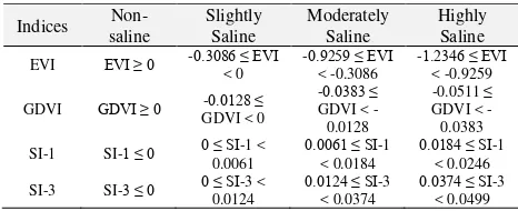
In thresholding method, high negative slopes of vegetation pixels and also high positive slopes of bare soil pixels are counted as highly saline lands. In contrast, the low-slope pixels are considered as slightly or non-saline. Accordingly, the slope maps of pixels, which were acquired from direct and indirect salinity indicators, were divided into four degrees of salinity based on maximum and minimum slope values which are: (1) non-saline, (2) slightly saline, (3) moderately saline, and (4) highly saline. Table 3 shows ranges of salinity classes for slope maps of selected indicators.
(a) (b)
(c) (d)
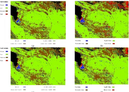
Figure 5. Map of salinity changes in vegetated lands based on pixel slopes during years 2000 to 2016, (a)EVI Slope, (b)K-Means on EVI Slope, (c) GDVI Slope and (d)K-Means on GDVI Slope.
(a) (b)
(c) (d)
Figure 6. Map of Salinity changes in bare soil lands based on pixel slopes during years 2000 to 2016, (a)SI-1 Slope, (b)K-Means on SI-1 Slope, (c) SI-3 Slope and (d)K-Means on SI-3 Slope.
Table 3. Ranges of salinity classes for slope maps of optimal algorithms which aims to find groups in the data (Trevino, 2016). The algorithm works iteratively to assign pixels to one of K clusters. In this study, four clusters were considered and slope maps of the study area were divided into four distinct classes. These classes represent degrees of salinity in the scene which were clustered based on similarity of pixel slopes. Since the algorithm does not recognize which cluster belongs to a certain salinity class, we determined classes manually using results of the thresholding method. The results of both methods to map salinity changes were compared with each other as shown in Figure 5 and Figure 6. We also assessed generated maps, which obtained by different salinity indicators, to determine the extent of salinization in both land cover classes of the study area
3.8 Discussion
Regarding the adverse impacts of saline soils on plantgrowth and also specific spectral reflectance characteristics of salt affected soils in satellite images, using different salinity indicators, which obtained from various band ratio combinations, is a suitable method to detect salinity and evaluate the rate of changes in multi-years studies in the absence of ground truth data. The most important point, in this case, is to select the best direct and indirect salinity indicators which have themost sensitivity to salt features in the study area.
In the case of vegetation, the results of the created map, which acquired from trend analysis of pixels in seventeen years, indicate that plants, which are close to the Bakhtegan Lake, are more affected by salinization. With increasing the distance from the lake, salinity decreased and vegetated areas changed slowly over years. These areas are slightly saline or even normal. Using optimal indices GDVI and EVI showed relatively same results. However, GDVI highlights changes more and salinity map indicates more pixels with high slope values. This can be due to the GDVI index formula which intensifies the differences between NIR and RED reflections.
In the case of bare soil lands, selected optimum indices SI-1 and SI-3 show the same spatial pattern of pixel changes and distribution of slope values in comparison with vegetated lands. Bare soil pixels with greater positive slopes, which represent highly salt affected soils, located near the salt Lake Bakhtegan. The more distance from the Salt Lake, the fewer changes in pixel values during 17 years. As it seen in Figure 6, most of the pixels were categorized to slightly and moderately saline which means that the study area is affected by salinity hazard. It can be expected that more regions around the lake will be in danger of salinization in next few years. Moreover, differences between generated slope maps of salinity indicators are negligible and the results are the same.
Evaluating the results of created maps by thresholding and K-means clustering methods shows that in both land covers, pixels with high slope values are located adjacent to the salt lake which
reveals that salts from the lake are brought into the soil and made changes to soils during 17 years especially in the areas around the lake. Although the pattern of changes in pixels is fairly similar in both methods, K-means clustering better highlights pixel variations and considers more pixels to highly salt affected the class. This can be observed in both vegetation and bare soil pixels. It can be concluded that using K-means clustering method, provides intensified results in comparison with Thresholding, therefore, pixels represent changes more and salinity classes were exaggerated. However, using thresholding method due to the possibility to determine accurate ranges of slopes for each salinity class is more reliable than K-Means method for this analysis.
Quantitative analysis of obtained slope values over 17 years, shows greater values of standard deviation in vegetation indices than salinity indices (Table 2) which can be due to higher variations of vegetation pixels in created slope maps. In addition, the range of slope values from salinity indices which were acquired from bare soil pixels shows fewer changes and are close to each other. It means that assessing soil salinity trends with regarding spectral behaviors of salt affected soils in bare soil lands is less impressive than using vegetation indices as indirect salinity indicators to evaluate plant loss. Moreover, increasing the spectral reflectance of soils over years may have other reasons.
4. CONCLUSION
This paper aims to assess trend analysis of soil salinity in different land cover types using the potential of satellite imagery. For this purpose, the area around the Bakhtegan Salt Lake was considered and two main land cover classes (vegetation, bare soil) were delineated to be analyzed separately. Salinity slope maps, which represent the rate of changes for each pixel in the scene, were generated for both land covers over years 2000 to 2016 using Landsat time series data along with optimum salinity indicators. High absolute values of slopes in both vegetation and bare soil lands correspond to highly salt affected regions. In contrast, fewer slope values represent slightly saline lands or non-saline. Accordingly, the study area was divided into four distinct salinity classes which are: (1) normal (healthy) soil, (2) slightly saline, (3) moderately saline, and (4) highly saline. The results indicate that the areas which are close to the salt lake in both lands cover more affected by salinization during 17 years study. It can be concluded that larger areas will be in danger of salinity hazard in next few years which should be considered in land management studies to prevent the destruction of natural resources and irrecoverable environmental damages. salinity using soil salinity and vegetation indices derived from IKONOS high-spatial resolution imageries: Applications in a date palm dominated region. Geoderma 230–231, 1–8. doi:10.1016/j.geoderma.2014.03.025 Azabdaftari, A., Sunar, F., 2016. Soil Salinity Mapping Using
Multitemporal Landsat Data. ISPRS - Int. Arch. Photogramm. Remote Sens. Spat. Inf. Sci. 41B7, 3–9. doi:10.5194/isprs-archives-XLI-B7-3-2016
Dubovyk, O., Menz, G., Conrad, C., Kan, E., Machwitz, M., Khamzina, A., 2013b. Spatio-temporal analyses of cropland degradation in the irrigated lowlands of Uzbekistan using remote-sensing and logistic regression modeling. Environ.
Monit. Assess. 185, 4775–4790. doi:10.1007/s10661-012-2904-6
Elhag, M., 2016. Evaluation of Different Soil Salinity Mapping Using Remote Sensing Techniques in Arid Ecosystems, Saudi Arabia. J. Sens. 2016, e7596175. doi:10.1155/2016/7596175
Gorji, T., Sertel, E., Tanik, A., 2017. Monitoring soil salinity via remote sensing technology under data scarce conditions: A case study from Turkey. Ecol. Indic. 74, 384–391. doi:10.1016/j.ecolind.2016.11.043
Imanyfar, S., Hasanlou, M., 2017. Remote sensing analysis of the extent and severity of oak decline in Malekshahi city, Ilam, Iran. Eng. J. Geospatial Inf. Technol. 4, 1–19. Ji-hua, M., Bing-fang, W., 2008. Study on the crop condition
monitoring methods with remote sensing. Int. Arch. Photogramm. Remote Sens. Spat. Inf. Sci. 37, 945–950. Ivushkin, K., Bartholomeus, H., Bregt, A.K., Pulatov, A., 2017.
Satellite Thermography for Soil Salinity Assessment of Cropped Areas in Uzbekistan. Land Degrad. Dev. 28, 870– 877. doi:10.1002/ldr.2670
Metternicht, G.., Zinck, J.., 2003. Remote sensing of soil salinity: potentials and constraints. Remote Sens. Environ. 85, 1–20. doi:10.1016/S0034-4257(02)00188-8
Metternicht, G., Zinck, A., 2008. Remote sensing of soil salinization: Impact on land management. CRC Press. Satir, O., Berberoglu, S., 2016. Crop yield prediction under soil
salinity using satellite derived vegetation indices. Field Crops Res. 192, 134–143. doi:10.1016/j.fcr.2016.04.028
Soil salinization [WWW Document], 2017. URL http://www.recare-hub.eu/soil-threats/salinization (accessed 5.6.17).
Trevino, A., 2016. Introduction to K-means Clustering [WWW
Document]. URL
https://www.datascience.com/blog/introduction-to-k-means-clustering-algorithm-learn-data-science-tutorials (accessed 5.7.17).
Wu, W., Mhaimeed, A.S., Al-Shafie, W.M., Ziadat, F., Dhehibi, B., Nangia, V., De Pauw, E., 2014. Mapping soil salinity changes using remote sensing in Central Iraq. Geoderma Reg. 2–3, 21–31. doi:10.1016/j.geodrs.2014.09.002
Scaramuzza, P., Micijevic, E., Chander, G., 2004. SLC Gap-Filled Products