Manajemen | Fakultas Ekonomi Universitas Maritim Raja Ali Haji 073500105000000171

(1)

Full Terms & Conditions of access and use can be found at

http://www.tandfonline.com/action/journalInformation?journalCode=ubes20

Download by: [Universitas Maritim Raja Ali Haji] Date: 12 January 2016, At: 23:23

Journal of Business & Economic Statistics

ISSN: 0735-0015 (Print) 1537-2707 (Online) Journal homepage: http://www.tandfonline.com/loi/ubes20

Testing Cross-Section Correlation in Panel Data

Using Spacings

Serena Ng

To cite this article: Serena Ng (2006) Testing Cross-Section Correlation in Panel Data Using Spacings, Journal of Business & Economic Statistics, 24:1, 12-23, DOI: 10.1198/073500105000000171

To link to this article: http://dx.doi.org/10.1198/073500105000000171

Published online: 01 Jan 2012.

Submit your article to this journal

Article views: 77

View related articles

(2)

Testing Cross-Section Correlation in

Panel Data Using Spacings

Serena N

G

Department of Economics, University of Michigan, Ann Arbor, MI 48109 (Serena.Ng@umich.edu)

This article provides tools for characterizing the extent of cross-section correlation in panel data when we do not know a priori how many and which series are correlated. Our tests are based on the probability integral transformation of the ordered correlations. We first split the transformed correlations by their size into two groups, then evaluate the variance ratio of the two subsamples. The problem of testing cross-section correlation thus becomes one of identifying mean shifts and testing nonstationarity. The tests can be applied to raw data and regression errors. We analyze data on industrial production among 12 OECD countries, as well as 21 real exchange rates. The evidence favors a common factor structure in European real exchange rates but not in industrial production.

KEY WORDS: Group effects; Purchasing power parity; Unit root; Variance ratio.

1. INTRODUCTION

Existing tests of cross-section correlation are concerned pri-marily with the null hypothesis that all units are uncorrelated against the alternative that the correlation is nonzero for some unit. Other statistics test group correlation in an error compo-nent framework and thus maintain identical correlation within group as the null hypothesis, assuming that group membership is known. But perfect and zero correlation are extreme hypothe-ses, and rejections by conventional tests do not always reveal much information about the extent of the correlation. It is often useful for estimation, inference, and economic interpretation to know whether a rejection is due to, say, 10% or 80% of the correlations being nonzero.

The present analysis is concerned with the situation when possibly some, but not necessarily all, of the units are corre-lated. The correlation is not sufficiently prevalent to be judged common, but is sufficiently extensive so that testing the no cor-relation hypothesis will almost always lead to a rejection. Our objective is to characterize the correlation without imposing a structure. This means determining the number of correlated pairs, determining whether the correlations are homogeneous, and evaluating the magnitude of the correlations.

We develop tools to assess the extent of cross-section correla-tion in a panel of data withNcross-section units andTtimes se-ries observations. Our analysis is based on then₌N_·(N₋1)/2 unique elements above the diagonal of the sample correlation coefficient matrix, ordered from the smallest to the largest. We do not directly test whether the sample correlations ( jointly or individually) are zero. Instead, we test whether the probabil-ity integral transformation of the ordered correlations, denoted byφ¯j, are uniformly distributed. If the underlying correlations are 0, then the “uniform spacings,” defined asφ¯j− ¯φj−1, is a

stochastic process with well-defined properties, and it is these properties that we test.

Exploiting the duality between uniformity and no correlation in hypothesis testing is not new. Durbin (1961) considered us-ing uniformity as a test for serial correlation in independent normally distributed data. The idea is that if the periodogram is evenly distributed across frequencies, then a suitably scaled periodogram is uniform on [0,1]. Here we use uniformity to test cross-section correlation.

We partition the spacings into two groups, labeledS(small) andL(large), withθˆ_{∈ [}0,1_]being the estimated fraction of the sample inS, and which we estimate using a breakpoint analy-sis. For each group, we test whether the variance ofφ¯j− ¯φj−q is linear inq. Essentially, the problem of testing cross-section correlation is turned into a problem of testing uniformity and nonstationarity. If we reject the no correlation hypothesis in the Lsample but not in theSsample, then we can say that a frac-tionθˆof the correlation coefficients are not statistically differ-ent from 0. This is unlike existing tests when a rejection often reveals little about the extent of the correlation. Our procedures are valid when applied to the full or a subset of the correlations, a property that conventional tests usually do not have. Because the identity of the series generating small and large correlations can always be recovered, knowing which correlation pairs be-long toScan sometimes reveal useful information for economic analysis.

The treatment of cross-correlation in the errors has impor-tant implications for estimation and inference. In recent work, Andrews (2003) showed that ordinary least squares, when ap-plied to cross-section data, can be inconsistent unless the errors conditional on the common shock are uncorrelated with the re-gressors. The usualttest will no longer be asymptotically nor-mal when there is extreme correlation, such as that induced by a common shock. Knowledge of the pervasiveness and size of the residual correlations is thus important.

Omitting cross-section correlation is known to create prob-lems for inference. Richardson and Smith (1993) noted that evi-dence for cross-sectional kurtosis could be the result of omitted cross-section correlation in stock returns. The panel unit root tests developed by Levin, Lin, and Chu (2002) and others are based on the assumption that the units in the panel are uncor-related. In a largeT, small N setup, O’Connell (1998) found that the much-emphasized power gain of panel over univariate unit root tests could be a consequence of omitted cross-section correlation, causing the panel tests to be oversized. The tests proposed by Moon and Perron (2004) and Bai and Ng (2004) are valid when the correlation is driven by a pervasive source.

(3)

Which test is appropriate depends on how many units are cor-related.

Recent years have seen much interest in using approximate factor models in econometric modeling. These differ from clas-sical factor models by allowing weak cross-section correla-tion in the idiosyncratic errors, where “weak” is defined by a bound on the column sum of theN_×N covariance matrix of the idiosyncratic errors (see Stock and Watson 2002; Bai and Ng 2002). However, this definition of weak cross-section correlation, although useful for the development of asymptotic theory, is not useful in guiding practitioners as to how much residual correlation is in the data. Toward this end, this arti-cle provides agnostic tools for identifying and characterizing correlation groups. The procedures can be applied to test cor-relations for which√T-consistent estimates are available. The article proceeds with a review of tests for cross-section corre-lation in Section 2. The procedures are developed in Sections 3 and 4, and simulations are reported in Section 5.

2. RELATED LITERATURE

Suppose that we haveNcross-section units each withTtimes series observations. Denote theT_×N data matrix byz. This could be raw data or, in regression analysis, z would be the regression errors. We are interested in characterizing the cross-correlation structure ofzit. Write

zit=δiGt+eit, (1)

where E(eit)=0 and E(eitejt)=ωij. The N ×N population variance–covariance matrix of z with var(Gt) normalized to unity is

z=δδ′+,

where(whosei,jelement isωij) will generally be nonspher-ical because of cross-section correlation and/or heteroscedas-ticity ineit. Ifδi=0 for alliandωij=0 ifi=j, thenzis a

diagonal matrix, and the data are cross-sectionally uncorrelated. Strong-form cross-section correlation occurs when|δi| =0 for almost everyiand the largest eigenvalue ofis bounded so that all series are related through the common factor,Gt. The error-component structure occurs as a special case whenδi= ¯δ=0 for every i and₌ω2In. The presence of a common factor does not imply that all bivariate correlations will be identical, because this will depend on the factor loadingδi, as well as on the importance of the idiosyncratic error,eti. We are especially interested in better understanding the intermediate cases when the two extremes of zero and strong correlation are inappropri-ate characterizations of the data.

Let cij=cov(zi,zj)/var(zi)var(zj) be the population cor-relation coefficient between two random variables, zi and zj. Given observations{zit}and{zjt},t=1, . . . ,T, the Pearson cor-relation coefficient is

ˆ cij=

sij √_s

iisjj

,

withsij=T−1Tt=1(zit− ¯zi)(zjt− ¯zj). If the data are normally distributed, thencˆit√(T−1)/

√

1− ˆc2_ijhas atdistribution with

T₋2 degrees of freedom under the null hypothesis of no cor-relation, and whenTis large,

√

T(_ˆcij−cij)≈N

0, (1−c2_ij)2.

Exact tests for equality of a set of correlation coefficients are available for normally distributed data because under normal-ity, expressions for the covariance of correlation coefficients are known. Otherwise, the asymptotic covariance of correlation co-efficients can be approximated by the delta method and shown to be a function of the true underlying correlations (see Olkin and Finn 1990; Steiger 1980; Meng, Rosenthal, and Rubin 1992). Under normality and assuming thatNis fixed, Breusch and Pagan (1980) showed that a test for the hypothesis that all correlation coefficients are jointly 0 is

LM=

N 2

−1 N

i=2 i₋1

j=1

Tc_ˆ2_ij_→χ_n2, (2)

with n₌N(N₋1)/2. When N is large, the normalized test

LM_√₋n

2n is asymptotically N(0,1)as T→ ∞and thenN→ ∞. A statistic that pools thepvalues is also asymptotically valid.

The LM test is asymptotically nuisance parameter-free when Tis large, but it depends on the properties of the parent distribu-tion even under the null hypothesis whenTis fixed. Using rank correlations, Frees (1995) considered a nonparametric test of no cross-section correlation in panel data whenNis large relative to T. A simulation based test was considered by Dufour and Khalaf (2002) for the null hypothesis that the error matrix from estimating a system of seemingly unrelated regressions with normally distributed errors is diagonal. Like the test of Frees and the LM test, the null hypothesis iscij=0 for all(i,j)pairs, and the test rejects whencij=0 for some(i,j)pair. At the other end of the spectrum, Moulton (1990) developed a test to detect group effects in panel data assuming that group membership is known (see also Moulton 1987). The maintained assumption is identical correlation within the group.

All of the aforementioned tests amount to testing zero or strong correlation. Only in rare cases can we test a correlation pattern other than the two extremes. The need to impose a rigid correlation pattern (i.e.,zis diagonal or has a factor structure)

in estimation and inference arises from that fact that unlike time series and spatial data, cross-section data have no natural or-dering. Absent extraneous information, the correlation with the neighboring observation has no meaningful interpretation. One cannot impose some type of mixing condition to justify testing the correlation among just a few neighboring observations.

From a practical perspective, the shortcoming of these tests is that rejecting the null hypothesis does not reveal much infor-mation about the strength and prevalence of the cross-section correlation. Whether the rejection is due to 10% or 80% of the correlations being nonzero makes a difference not just in the way we handle the correlation econometrically, but also in the way we view the economic reason for the correlation.

3. THE ECONOMETRIC FRAMEWORK

We start with the premise that the panel of data are neither all uncorrelated nor all correlated with each other. As a mat-ter of notation, we let [x_] denote the integer part ofx. For a

(4)

series xj,j=1, . . . ,n, letx[1:n],x[2:n], . . . ,x[n:n] denote the

or-dered series, that is, x_[1:n] =minj(xj) and x[n:n]=maxj(xj). We assume for now that the data are normally distributed and discuss the case of nonnormal data in Section 5. Because the analysis applies to other definitions of cross-section correlation coefficients, we generically denote the vector ofuniquesample correlation coefficients bypˆ and the corresponding population correlation coefficients byp. We also letp¯_{= |ˆ}p_|, the vector of absolute sample correlation coefficients. Thus if Pearson corre-lation is used for the analysis, then we have

ˆ

p₌(p_ˆ1,pˆ2, . . . ,pˆn)=vech(ˆc)

and

¯

p₌(_|ˆp1|,|ˆp2|, . . . ,|ˆpn|), n=N(N−1)/2.

We are interested in the severity of the correlation among the units. Our general strategy is to split the sample into a group of “small” and a group of “large” correlations, then test whether the small correlations are 0. The two steps allow us to under-stand how pervasive and how strong the cross-section correla-tion is.

The following lemma forms the basis of our methodology.

Lemma 1. Let (u1,u2, . . . ,un)′ be an n×1 vector of iid U[0,1]variates and letu_[1:n], . . . ,u[n:n]denote the ordered data.

LetD1=u[1:n],Dj=u[j:n]−u[j−1:n],j=2, . . . ,n, andDn+1=

1−u_[n_:n_] be the spacings. ThenE(Dj)= _n₊1₁, var(Dj)=n×

(n₊1)−2(n₊2)−1_∀j, and cov(Di,Dj)=₍_n₊₁−₎21₍_n₊₂₎ ∀i=j.

Ifujis uniformly distributed on the unit interval, then a plot ofjagainstu_[j:n]should be a straight line with slope 1/(n+1). units and the covariance between any two units are the same. (See Pyke 1965 for an excellent review on spacings.) We make use of the fact that if uj∼U[.5,1], then 2uj−1 is also uni-formly distributed on the interval[0,1], and spacings for 2uj−1 have the properties stated in Lemma 1. Because the spacings for uj∼U[.5,1]are half the spacings for 2uj−1, Lemma 1 implies

3.1 Partitioning the Correlations Into Two Sets

UnderH0:pj=0,

that is,p¯j is asymptotically distributed as chi (not chi-squared) with 1 degree of freedom, or, equivalently, √Tp_¯j is a half-normally distributed random variable with mean .7979 and vari-ance .3634. Sortp¯ from the smallest to the largest, and denote the ordered series by (p_¯_[1:n], . . . ,p¯[n:n])′. Taking absolute

val-ues ensures that large negative correlations are treated symmet-rically as large positive correlations. Defineφ¯jas(

√ Tp_¯_[j:n]),

whereis the cumulative distribution function of the standard

normal distribution. We have in principle at test can be constructed. But like the LM test, a rejection reveals little about the extent of the correlation.

Let φ¯j = ¯φj − ¯φj−1 be the spacings and, by Lemma 1,

Now suppose that only m_≤ n of the correlation coeffi-cients are 0 or small. We would expect φ¯j, j=1, . . . ,m, to be strictly less than 1. In contrast, we would expect the φ¯j, j₌m₊1, . . . ,n, to be close to 1 because ifp_[j+1:n]is not small,

then√Tp_¯_[j₊1_:n_]will diverge. In a q–q plot, we would expectφ¯j to be approximately linear injuntilj₌m, then rise steeply, and eventually flatten out at the boundary of 1. Letθ₌m/n. Then

The difference between¯Sand¯Lis thus informative aboutm, which we can estimate by locating a mean shift inφ¯jor by a slope change inφ¯j. Because we will be analyzing the properties ofφ¯jin the two subsamples, we look for a mean shift inφ¯j. Define the total sum of squared residuals evaluated at ˜

In our analysis, the series of ordered absolute values of the pop-ulation correlation coefficients, |p_[j:n]|, exhibits a slope shift

atm. Butp¯_[j:n]is√T-consistent for|p[j:n]|, andφ¯jis monotone-increasing in p¯_[j_:n_]. The criterion function Qn(θ )˜ converges uniformly to a function with a minimum where the true change-point in|p_[j:n]|occurs. Thus the global minimizer of (3), that is,

consistently estimates the break fractionθ, and the convergence rate isn(see Bai 1997). Partitioning the sample atm_ˆ _{= [ ˆ}θn_]is optimal in the sense of minimizing (3).

The foregoing analysis is designed for cases where a subset of the correlations are nonzero. But when all of the correlations

(5)

are large and close to unity, there will be no variation inφ¯j, and hence we would not expect to detect a mean shift inφ¯j. The foregoing breakpoint analysis, although informative, is incom-plete. To learn more about the nature of the correlation, such as whether the correlations are homogeneous or heterogeneous, we need to go one step further. Before proceeding with such an analysis, we first illustrate the properties of the breakpoint estimator using some examples.

3.2 Illustration

We simulate data as follows. For each i ₌ 1, . . . ,N, t₌1, . . . ,T,

zit=δiGt+eit and

et=(e1t, . . . ,eNT)′∼1/2N(0N,IN),

whereGt∼N(0,1)and1/2is an×nmatrix. By varying the number ofδithat are nonzero or the structure of1/2, we have 10 configurations representing different degrees of correlation in the data.

DGP 1 simulates a panel of uncorrelated data. DGPs 2 and 3 assume the presence of a common factor but with different as-sumptions about the importance of the common to idiosyncratic component. DGP 4 and 5 assume that1/2is a Toeplitz matrix but the δi’s are all 0. (A Toeplitz matrix is a band-symmetric matrix.) Under DGP 5, the diagonal elements of1/2are 1, the elements above and below the diagonals are .8, and all other elements are 0. Under DGP 6, the diagonal elements of1/2

are 1, those above and below the diagonal elements are₋.5, the elements that are two positions from the diagonal are .3, and all other elements are 0. DGPs 6 and 7 assume equal corre-lation within a group but with varying group size. DGPs 8–10 make different assumptions about the number of δi’s that are nonzero. Because δi varies across i, there is heterogeneity in the magnitude of the correlation.

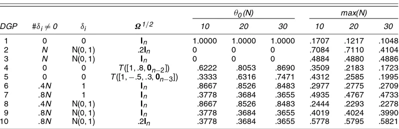
Defineθ0as the fraction of zero entries above the diagonal of

theN_×Nmatrixz. In general,θ0will be different thanθ, the

fraction of correlated pairs that are small. As a benchmark for how correlated the data are, Table 1 reportsθ0forN=10,20,

and 30. Notice that under DGP 5 and 6,θ0varies withN. This

is because the number of nonzero entries inincreases with the number of nonzero entries in1/2in a nonlinear way. The “max”column reports maxi_N1Nj₌1|ˆcij| in 1,000 replications. This statistic is an upper bound on the average correlation in the data because from matrix theory, the largest eigenvalue ofzis

bounded by maxjni=1|cij|. The bound is often used as a con-dition on permissible cross-section correlation in approximate factor models (see, e.g., Bai and Ng 2002; Stock and Watson 2002). However, this statistic has shortcomings as a measure of severity of the correlations in the panel of data. For one thing, “max” is not monotonic in the number of nonzero correlations; for example, DGP 3 has more nonzero correlations than DGP 10, yet “max” is larger in DGP 10 than in DGP 3. For another, two similar values of “max” can be consistent with very differ-ent degrees of correlatedness; for example, DGPs 5 and 6 both have similar “max” values whenN₌20, butθ0is much higher

under DGP 6. The point to highlight is that when there is hetero-geneity in the correlations, it will be difficult to characterize the severity of the correlation with a single statistic. This is unlike the situation for time series data, where the largest root of the autocorrelation matrix is informative about the extent of serial correlation.

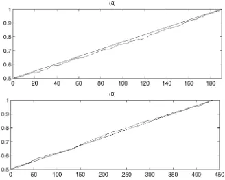
Many of the features aboutφ¯j can be illustrated by looking at the q–q plot for a particular draw of the data. Figure 1(a) considers DGP1 (uncorrelated data) for T₌200 and N₌20 (or n₌190); Figure 1(b) considers T₌400 and N₌30 (or n₌435). Figure 1 depicts the line .5+.5j/(n₊1)on which all φ¯j should lie if they are exactly uniformly distributed. In finite samples, φ¯j should be approximately linear in j if they are transformed from normally distributed variables. Because the data are uncorrelated, the quantile function does not exhibit any abrupt change in slope, and the average ofφ¯jis approxi-mately ₂₍_n1₊₁₎.

Now consider the case of correlated data generated by DGPs 9 and 10. In both cases, about one-third of the correlations are 0, but the correlations are much smaller (and hence φ¯j) under DGP 9 because of the larger idiosyncratic variance. Be-cause many correlations are nonzero, Figure 2 shows thatφ¯jno longer evolves around the straight line with slope ₂₍_n1₊₁₎. In-stead, a subset of them vary around a straight line drawn with anx-axis that is appropriately truncated to the number of corre-lation coefficients that are 0 or small.

For the sample of data simulated using DGP 9, 82 of theφ¯j’s are <.95. This means that if we used the asymptotic standard error under no correlation of √1

T to test the 190 correlations one by one, then we would end up with a groupSconsisting of 82 correlations deemed insignificant at the 5% level. A differ-ent significance level will produce a differdiffer-ent group size. Our breakpoint analysis does not depend on the choice of the sig-nificance level; rather, it lets the data determine the sharpest difference between the two groups.

Table 1. DGP

θ0(N) max(N)

DGP #δi=0 δi Ω1/2 10 20 30 10 20 30

1 0 0 In 1.0000 1.0000 1.0000 .1707 .1217 .1048 2 N N(0, 1) .2In 0 0 0 .7084 .7110 .4104

3 N N(0, 1) In 0 0 0 .4884 .4880 .4886

4 0 0 T([1, .8,0_n₋₂]) .6222 .8053 .8690 .3509 .2183 .1723 5 0 0 T([1,₋.5, .3,0_n₋₃]) .3333 .6316 .7471 .4312 .2585 .1995 6 .4N 1 In .8667 .8526 .8483 .2977 .2775 .2709

7 .8N 1 In .3778 .3684 .3655 .4935 .4767 .4733

8 .4N N(0, 1) In .8667 .8526 .8483 .2444 .2293 .2278

9 .8N N(0, 1) In .3778 .3684 .3655 .4019 .4024 .3990

10 .8N N(0, 1) .2In .3778 .3684 .3655 .5778 .5795 .5821

(6)

(a)

(b)

Figure 1. φ¯(j): DGP 1. (a) T=200, N=20; (b) T=400, N=30.

Figure 3 presents φ¯j for DGP 2 (small idiosyncratic error) and 3 (large idiosyncratic error). Because DGP 2 has a stronger factor structure than DGP3, there are moreφ¯j’s at unity. In both cases, the minimum φ¯j is >.5, indicating even the small cor-relations are nonzero. The feature to highlight in Figure 3 is that pj can be nonzero and yetφ¯j<1. We cannot always use the boundary of 1 to split the sample. Instead, we use the least squares criterion to separate the small and large correlations.

Figures 1, 2, and 3 show that the q–q plot indeed reveals much information about the extent of cross-correlation in the data. If all correlations are nonzero, then the q–q plot will be shifted upward with an intercept exceeding .5. If there is

homo-Figure 2. φ¯(j): DGPs 1 ( ), 9 ( ), and 10 ( ). Here zit=δiGt+eit,

δi ∼N(0, 1), i=1, . . . ,.8N=152, and δi=0, i>.8N. For DGP 9,

e_it_∼N(0, 1). For DGP 10, e_it_∼N(0, .2).

geneity in a subset of the correlations, then the q–q plot should be flat over a certain range, because there is no dispersion in the correspondingφ¯j’s. The more prevalent and the stronger the correlation, the further away areφ¯j from the straight line with slope₂₍_n1₊₁₎.

4. TESTING THE CORRELATION IN THE SUBSAMPLES

So far, we have used the breakpoint estimator to split the sample ofn observations into two groups, one of size mˆ and the other of sizen_{− ˆ}m. It is possible that then_{− ˆ}mcorrelations

Figure 3.φ¯(j): DGPs 1 ( ), 2 ( ), and 3 ( ).φ¯jcan be<1 even though

DGPs 2 (small idiosyncratic errors) and 3 (large idiosyncratic errors) both have a factor structure.

(7)

inLare, in fact, not statistically different from themˆ correla-tions inS. Verifying this by testing the null hypothesis of no break is uninformative, because an error component structure would be consistent with the no break hypothesis as all correla-tions are identical, and yet incompatible with the no correlation assumption. In theory, it is also possible to formulate an order-statistic–oriented test based on the idea that all nonzero corre-lations, when multiplied by√T, are “large” with probability 1. But, as we have seen, some nonzero correlations may not be large enough to renderφ¯jexactly 1. Applying an LM test to the subsamples is also problematic, becausep_¯_[j_:n_],j=1, . . . ,mˆ, is a censored sample whenevermˆ <n. The subsample test will no longer be asymptotically chi-squared.

Here we consider a different approach that aims to test whether the subset of mˆ correlations are 0. If the small cor-relations are found to be different than 0, then the corcor-relations inLmust also be different than 0.

Lemma 2. Let uj∼U[0,1] with Dj=u[j:n]−u[j−1:n]

be-ing uniform spacbe-ings. Then (a)nDj∼Ŵ(1,1)and (b) corr(nDj, nDk)=−_n1 ∀j=k. LetDq_j =u_[j_:n_]−u_[j₋q_:n_]beq-order spac-ings. Then (c)Dq_j _∼beta(q,n₋q₊1)and (d)nDq_j _∼Ŵ(q,1).

The simple spacings, multiplied by n, are distributed as Ŵ(1,1). Although the spacings are not independent, they are asymptotically uncorrelated. Furthermore, the structure of de-pendence is the same betweenDjandDkfor anyjandk. Spac-ings are thus “exchangeable.” The quantityu_[j:n]−u[j−q:n] is

referred to in the statistics literature as aq-order spacing. Prop-erties ofq-order spacings have been given by Holst (1979) and Arnold, Balakrishman, and Nagaraja (1992).

The features that motivate the test that follows are (a) and (d). Property (a) implies that if we define

¯

φn_j ₌n_{· ¯}φj,

and again using the fact that the spacings of variables that are uniformly distributed on[.5,1]are half of the uniform spacings, then we can represent the scaled spacings processφ¯_jnas

¯

n . Viewed in this light, ¯

φn_j is a unit root process with a nonzero drift that tends to .5 whenN_{→ ∞}.

The observation thatφ¯n_j is a differenced stationary process is reinforced by (d), which states that the mean and variance of q-order spacings are _n₊q₁ and ₍_nq(n+1−q)

+1)2₍_n₊₂₎. But this implies

that the mean and variance ofqorder spacings areqtimes the mean and variance of the scaled order spacings. A first-order integrated process also has this variance ratio property.

The feature thatφ¯_jnis differenced stationary originates from the property thatφ¯j is uniformly distributed under the no cor-relation assumption. Evidence against nonstationarity ofφ¯_jn is thus evidence against no cross-section correlation. Thus we can use methods for analyzing integrated data to test cross-section correlation. Consider testing the no correlation hypothesis us-ing a vector ofφ¯_kn of dimensionη; for example,η_{= ˆ}mif we

were to test the hypothesis of no correlation in the subsampleS. Let

(1₋q/η), which will yield an unbiased estimate of the variance. Define To gain more intuition, letq₌2 and consider

ˆ

The first ratio on the right side is the first-order autocorrelation coefficient forφ¯n_j, whereas the second term in the numerator is the squared difference between the mean ofq-order and sim-ple spacings. But by (b) of Lemma 2, φ¯_jn is asymptotically uncorrelated, and by (a) of Lemma 2, the mean ofqorder spac-ings is linear inq. Both terms on the right side should be close to 0. A comparison ofσˆ_q2toσˆ₁2thus allows us to test both prop-erties of spacings that should hold if the underlying correlations are indeed 0.

Theorem 1. Consider the null hypothesis that a subset of p_[j:n] of size η are jointly 0. Then, as η→ ∞, √η×

SVR(η)_−→d N(0, ω2_q), whereω2_q₌2(2q−₃1_q)(q−1).

Various authors have used functions of simple andq>1 or-der spacings to test uniformity. Rao and Kuo (1984), among others, showed that using squares of the spacings in testing is optimal in terms of maximizing local power. Our spacings variance ratio (SVR) test is also based on the second moment of spacings. In the statistics literature, σ_ˆ₁2 and q_{· ˆ}σ_q2 are re-ferred to as simple and generalized Greenwood spacing tests for uniformity. The original Greenwood statistic was developed to test whether the spread of disease is random in time. Wells, Jammalamadaka, and Tiwari (1992) showed that spacing tests have the same asymptotic distribution when parameters of the distribution to be tested must be estimated as when the parame-ters are known. We combine the simple Greenwood test with aq-order test and apply our test to functions of estimated cor-relations, not the raw data. As shown in the Appendix, we can treat theφ¯j’s as though they are uniformly distributed on[.5,1], provided thatT_{→ ∞}.

The limiting distribution of the SVR test is obtained by noting that σˆ₁2 andσˆ_q2 are both consistent estimators for σ_ǫ2,

(8)

but σˆ₁2 is efficient. Thus the Hausman principle applies, and var(σ_ˆ_q2_{− ˆ}σ₁2)₌var(σ_ˆ_q2)₋var(σ_ˆ₁2), from which var(σ_ˆ_q2/σ_ˆ₁2₋1) is obtained. In actual testing, we use the standardized SVR test, that is,

which in large samples is asymptotically standard normal. Some might observe that the SVR test has the same limiting distribution as the variance ratio (VR) test of Lo and MacKinlay (1988) for testing the null hypothesis of a random walk, that is, with ǫj ∼N(0, σ2). The ǫj’s considered here are nonnormal, however. Although the kurtosis ofφ¯jappears in the variance of

ˆ

σ₁2 andσˆ_q2, the two kurtosis terms offset one another because we consider the variance of the difference. At an intuitive level, the reason that the SVR has the same distribution as the VR is that we are testing whether the variance ofqφ¯_jnis linear inq. This is a property of an integrated process, not just that of a random walk with Gaussian innovations.

The SVR test can be constructed in slightly differently ways. For example, one can follow the Greenwood statistic and setµ_ˆ1

to the population mean, which amounts to.5 in our setup, or one can setµˆqtoqµˆ1as in the VR test. Becauseµˆ1consistently

estimates the mean of .5, andµ_ˆqandqµˆ1are both consistent for

the mean ofq-spacings under the null, the limiting distribution of the SVR test is the same for all implementations.

The SVR test can be applied to the full sample, to S, or toL, withη₌n,η_{= ˆ}m, or η₌n_{− ˆ}m. An important appeal of the SVR test is that it is based on spacings, and spacings are exchangeable. That is, we can test any subset of the spac-ings between adjacent order statistics. As seen in Figure 1 for uncorrelated data, the φ¯j’s all lie along the straight line. This allows us to use any partition of the full sample to test the slope. Obviously, if we reject the uniformity hypothesis inS, then testing whether the hypothesis holds inLis not too inter-esting because, by construction,Sis the sample with the smaller correlations. But in principle we can reapply the breakpoint es-timator to the partitionSto yield two subsamples withinS, say SSandSL. We then can perform the SVR test to see whether the subsampleSSconsists of uncorrelated coefficients. In contrast, the LM test loses its asymptotic chi-squared property once the sample is censored. But there are two caveats to repeatedly ap-plying the proposed procedures. First, if there are already too few observations inS, then the subsampleSSmay be too small to make the tests precise. Second, if the SVR is applied to the SSsubsample after theSsample rejects uniformity, then the se-quential nature of the test would need to be taken into account. Because the identity of the two series underlying any givenp_¯j can always be recovered, the procedure can be used to see whether those highly correlated pairs share common charac-teristics. It should be noted, however, that correlations are not transitive; that is, cov(zi,zj)=0 and cov(zj,zk)=0 do not nec-essarily imply cov(zi,zk)=0. Our analysis provides a classi-fication of correlation pairs into groups. Additional economic analysis is needed to determine whether the series underlying the correlation pairs can be grouped.

5. FINITE–SAMPLE PROPERTIES

For each of the 10 models given in Table 1, we consider (N,T)₌(10,100), (20,100), (20,200), and (30,200). In

re-sults not reported here, an LM test for the null hypothesis that pj=0 for alljas well as attest forE(φj)=.75 have a rejec-tion rate of 1 when tested on DGPs 2–10. These rejecrejec-tions are uninformative about the extent of the cross-section correlation, however.

Besides the Pearson correlation, we also use other measures forpˆj. LetRibe aT×1 vector of rankings ofzit. The Spearman rank correlation coefficient is defined as

ˆ 1)/2) is the sample covariance in the rankings of two series, zitandzjt. It is well known that√(T−2)· ˆrij/

√

1− ˆr2_ij_∼tT−2.

The statistic has mean 0 and variance T_T−₋3₅, which becomes approximately unity as T _{→ ∞}. We also consider Fisher’s z-transformation of the Pearson correlation coefficient,

ˆ cially useful in stabilizing the variance whenT is small. Anal-ogously, a transformation can also be applied to the Spearman rank correlations and Kendall’sτ.

To summarize, givenN cross-section units overT time pe-riods with n₌N(N₋1)/2, the following variables are con-structed:

ˆ

cij(z): sample cross-section correlations ˆ

Tables 2 and 3 report results for the Pearson correlation co-efficients assuming thatǫitis normally distributed. Results for Fisher’szcorrelations are given in Tables 4 and 5. Results for the Spearman rank correlations are similar and hence are not reported here. The sample correlations are estimated more pre-cisely the larger theT, although the sample-splitting procedure is more accurate the larger theN. Because it is difficult to iden-tify mean shifts occurring at the two ends of the sample, we use 10% trimming; that is, the smallest and largest 10% ofφ¯j are not used in the breakpoint analysis. Recall thatθˆestimates the fraction of “small” correlations. The average and the standard deviation ofθˆ over 1,000 replications are reported in columns three and four. Given that we use 10% trimming, having an av-erageθˆ of around .1 for DGP 2 is clear evidence of extensive correlation. The average θˆ is around .3 for DGP 3. The rea-son that DGPs 2 and 3 have rather differentθˆ’s even though theθ0’s are the same is that DGP 3 has higher idiosyncratic

er-ror variance. Consequently, more correlations are nonzero, al-beit small. This again highlights the point thatθ0(the fraction

of zero correlations) need not be the same asθ (the fraction of small correlations). Althoughθ0is a useful benchmark,θis

more informative from a practical perspective, and an estimate ofθis provided by our breakpoint analysis.

(9)

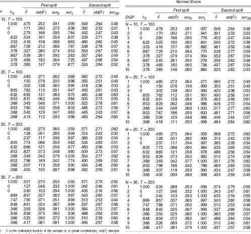
Table 2. Pearson Correlation Coefficients: Normal Errors 10 .366 .417 .081 .081 1.000 .495 .257 .058

NOTE: θˆis the estimated fraction of the sample inS(small correlations). std(θˆ) denotes the standard deviation ofθˆin 1,000 replications.svrSandsvrare the rejection rates of the standardized spacings variance-ratio test applied to the subsamplesSandL.

Next, we apply thesvrtest to the two subsamples withq₌2. The critical value for a two-tailed 5% test is 1.96. The results are based on 1,000 replications. The rejection rates are labeled svrSandsvrL. The rejection rate should be .05 in both subsam-ples of DGP 1, because the data are uncorrelated. The test is oversized when(N,T)₌(10,100)but is close to the nominal size of 5% for larger(N,T). The size distortion whenN₌10 is due to the small size of the subsamples (which have<25 obser-vations given thatθˆis, on average, around .5). For DGPs 2–10, thesvrL tends to reject uniformity with probability close to 1 whenN₌20, demonstrating that the test has power. Because the correlations in theLsubsample are large by selection, the ability to reject uniformity inLis not surprising. It is more dif-ficult correctly reject uniformity inSwhen the underlying cor-relations are small but not necessarily 0. The size of the test is generally accurate, especially considering the average size of the subsamples. We also splitS into two samples,SSandSL,

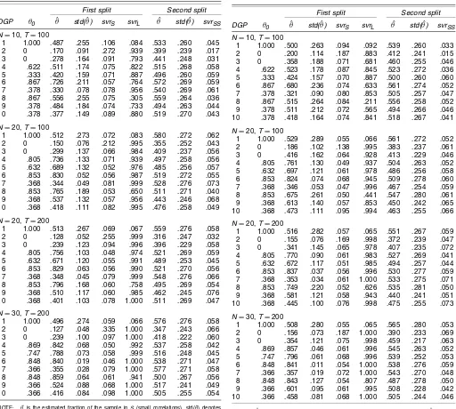
Table 3. Fisher-Transformed Pearson Correlation Coefficients: Normal Errors 10 .366 .417 .081 .079 1.000 .497 .257 .058

and then apply the svr to SS. Table 3 shows that the rejec-tion rates are generally similar to those using the larger sam-ple,S, demonstrating that censoring poses no problem for the spacings-basedsvr.

Strictly speaking, Lemmas 1 and 2 apply to iid uniform vari-ables. Except when the data are normally distributed, the sam-ple correlations are not independent. Nonetheless, even when the data are nonnormal,cˆij is at least asymptotically normally distributed and hence asymptotically independent. The spac-ings thus should be independently uniformly distributed in large samples. We can use simulations to check robustness of the results against departures from normality in finite samples. Table 4 reports results for Pearson correlations assuming that ǫit is a chi-squared variable with 1 degree of freedom. Table 5 assumes thatǫit is a ARCH(1)process (with parameter .5). As we can see, the breakpoint analysis and thesvrtest have

(10)

Table 4. Pearson Correlation Coefficients: ARCH(1) Errors 10 .368 .401 .103 .078 1.000 .511 .269 .047

N=30,T=200 10 .366 .416 .084 .098 1.000 .505 .255 .054

ties similar to those reported in Tables 2 and 3. This robustness to departures from normality is likely due to the fact that the breakpoint analysis is valid under very general assumptions, and the SVR tests a generic feature of integrated data. Thus both the breakpoint analysis and the SVR test continue to have satisfactory finite-sample properties.

5.1 Applications

We consider two applications. The first analyzes the corre-lation in real economic activity in the Euro area, and the sec-ond considers a panel of real exchange rate data. To isolate cross-section from serial correlation, we compute the correla-tion coefficients for residuals from a regression of each variable of interest on a constant and its own lags.

Industrial Production. Letzit,i=1,12,t=1982:1–1997:8, be monthly data on industrial production for Germany, Italy,

Table 5. Pearson Correlation Coefficients:χ₁2Errors

First split Second split 10 .366 .458 .081 .068 1.000 .505 .244 .046

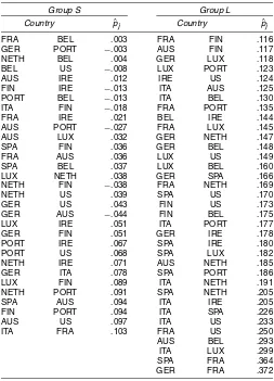
Spain, France, Austria, Luxembourg, the Netherlands, Finland, Portugal, Belgium, Ireland, and the United States. These data are the same as given by Stock, Watson, and Marcellino (2003). With 12 countries, we haven₌66 forT ₌186 observations. The variable of interest is the growth rate of industrial produc-tion. Figure 4 plotsφ¯j. Although most of theφ¯j’s are far from unity, the observations do not lie along a straight line, indicat-ing substantial heterogeneity in the correlations. The breakpoint analysis yieldsθˆ₌.468, 31 correlations inS, and 35 correla-tions inL. Thesvrtest statistics are−.234 and 2.673. Industrial production in 31 of the 66 country pairs appear to be contem-poraneously uncorrelated. Because there are many zero corre-lation pairs, a common factor structure does not appear to be a suitable characterization of the output of these 12 countries.

A listing of the correlations in the two groups is given in Table 6. The largest correlation is the France–Germany pair

(11)

Figure 4. φ¯(j): Growth Rate of Industrial Production for 12 OECD Countries.

(p¯j=.33), and the weakest is between Austria and Luxem-bourg (p¯j=.006). As pointed out by a referee, France is highly correlated with Belgium, which is highly correlated with Spain, but the correlation between Spain and Belgium is in the low group. This result, which is of some economic interest, clearly

Table 6. Correlations in Industrial Production for 12 OECD Countries

Group S Group L

Country pˆj Country pˆj

FRA BEL .003 FRA FIN .116 GER PORT ₋.003 AUS FIN .117 NETH BEL .004 GER LUX .118 BEL US ₋.008 LUX PORT .123

AUS IRE .012 IRE US .124

FIN IRE ₋.013 ITA AUS .125 PORT BEL ₋.013 ITA BEL .130 ITA FIN ₋.018 FRA PORT .135 FRA IRE .021 BEL IRE .144 AUS PORT ₋.027 FRA LUX .145 AUS LUX .032 GER NETH .147 SPA FIN .036 GER BEL .148

FRA AUS .036 LUX US .149

SPA BEL .037 LUX BEL .160 LUX NETH .038 GER SPA .166 NETH FIN ₋.038 FRA NETH .169

NETH US .039 SPA US .170

GER US .043 FIN US .173

GER AUS ₋.044 FIN BEL .175 LUX IRE .051 ITA PORT .177 GER FIN .051 GER IRE .178 PORT IRE .067 SPA IRE .180 PORT US .068 SPA LUX .182 NETH IRE .071 AUS NETH .185 GER ITA .078 SPA PORT .186 LUX FIN .089 ITA NETH .191 NETH PORT .091 SPA NETH .205 SPA AUS .094 ITA IRE .205 FIN PORT .094 ITA SPA .226

AUS US .097 ITA US .233

ITA FRA .103 FRA US .250

AUS BEL .293 ITA LUX .299 SPA FRA .364 GER FRA .372

NOTE: The industrial production data are for Germany, Italy, Spain, France, Austria, Lux-embourg, the Netherlands, Finland, Portugal, Belgium, Ireland, and the United States for 1982:1–1997:8.

Figure 5. φ¯(j): Real Exchange Rates for 21 Countries.

shows that our analysis provides a way to classify correlation coefficients into groups. Economic analysis will be necessary to see whether the series underlying the correlations can be grouped meaningfully.

Real Exchange Rates. Quarterly data for nominal exchange rates and the consumer price indices were obtained from the In-ternational Finance Statistics. We use data from 1974:1–1997:4 for 21 countries: Canada, Austria, New Zealand, Australia, Belgium, Denmark, Finland, France, Germany, Ireland, Italy, Netherlands, Norway, Spain, Sweden, Switzerland, U.K., Japan, Korea, Singapore, and Thailand. The United States is used as the numeraire country. The variable of interest is the log real exchange rate.

A plot ofφ¯jis presented in Figure 5. The algorithm finds that ˆ

θ₌.142, so .85 of the sample belongs toL. Because there are a total of n₌210 correlations in this example, Table 7 gives only the 30 correlations in S and the 30 largest correlations inL. Evidently, correlations involving the real exchange rates for Canada and Korea do not display much correlation with those of the European countries. However, the European real exchange rates are strongly correlated with one another. The results suggest that one cannot simply attribute the source of the correlations to the use of a common numeraire (the U.S. dollar). If this were the sole source of the correlation, then all real exchange rates should be equally correlated.

Thesvrtest statistic withq₌2 is 1.884 for theSsample of size 30 and 8.574 for the Lsample. Withq₌4, these statis-tics test are 1.4585 forSand 10.8271 forS. Further partitioning the L sample yields asvr for LSof 8.5724. Evidence against no correlation in theLsample is compelling. BecauseL consti-tutes .85 of the correlation pairs, the cross-section correlation in the panel is extensive. Not accounting for these correlations when constructing panel unit root tests can indeed lead to mis-leading inference about persistence.

Putting the two sets of results together suggests stronger and more extensive correlation for the European real exchange rates than for industrial production. Indeed, the first principal compo-nent explains more than 60% of the variation in real exchange rates. Because a common factor exists in European real ex-change rates but not in real output, the evidence points to the presence of a nominal or a monetary factor.

(12)

Table 7. Real Exchange Rates for 21 Countries

Largest 30 correlations in group L Group S

Country pˆj Country pˆj

CAN FR .008 NETH NOR .847 CAN NETH .009 AUS IRE .851 CAN SPA .016 FR SWTZD .857 CAN GER .019 GER IRE .860 CAN ITA .020 BEL SWTZD .862 CAN BEL .021 BEL IRE .867 CAN NOR .025 DEN SWTZD .867 UK KOR ₋.026 DEN IRE .869 CAN AUS .030 IRE NETH .869 SWTZD KOR .045 FR IRE .870 CAN SWED .050 GER NOR .871 FIN KOR .050 AUS NOR .872 DEN KOR .052 AUS SWTZD .876 CAN SWTZD .052 NETH SWTZD .877 CAN SG .052 GER SWTZD .879 NETH KOR .053 DEN FR .913 SWED KOR .056 AUS FR .921

CAN IRE .056 BEL FR .922

CAN THAI .058 FR GER .922 ITA KOR .058 FR NETH .927

FR KOR .059 AUS DEN .950

BEL KOR .064 DEN GER .956 CAN JP .064 DEN NETH .959 GER KOR .065 BEL DEN .963 AUS KOR .068 AUS BEL .963 CAN DEN .070 BEL GER .964 IRE KOR .076 BEL NETH .970 NOR KOR .078 AUS NETH .978 CAN UK .081 GER NETH .982 SPA KOR .085 AUS GER .985

NOTE: The real exchange rates are for Canada, Australia, New Zealand, Australia, Bel-gium, Denmark, Finland, France, Germany, Ireland, Italy, Netherlands, Norway, Spain, Sweden, Switzerland, U.K., Japan, Korea, Singapore, and Thailand. The United States is used as the numeraire country. The sample is for 1974:1–1997:4.

6. CONCLUSION

This article has presented an agnostic way of testing cross-section correlation when possibly a subset of the sample is cor-related. This is a situation in which traditional testing of the no correlation hypothesis in the full sample is rejected, but for which the rejection provides little understanding about the ex-tent of the correlation. Our analysis makes use of the fact that if the population correlations are 0, then the spacings of the transformed sample correlations should have certain properties. We use a breakpoint analysis and a variance ratio test to assess

whether the properties of the spacings are consistent with the underlying assumption of zero correlation. We take a Gaussian transformation of|√Tp_¯_[j:n]|. An alternative is to definep˜[j:n]

as the sorted series ofpˆ2_j. Then a chi-squared transformation ofTp_˜_[j_:n_]should be approximately uniformly distributed on the unit interval. The results for uniform spacings can be applied immediately, and our main results will continue to hold.

APPENDIX: PROOFS

We need to show that the tests, which are based on trans-formations of the sample correlations, are unaffected by the sampling variability of estimated correlation coefficients. Let (_·) denote the standard normal distribution and zα be the α-level standard normal quantile, that is, (zα)=α. It is known that if a statistic τ_ˆ is √T consistent and asymptoti-cally normal, then Pr(τ_ˆ_≤zα)=(zα)+T−1/2′(zα)v1(zα)+

T−1v2(zα)′′(x)+ · · ·,wherevjis a polynomial. Furthermore, if Pr(τ_ˆ_≤qα)=α, then the quantileqα admits the expansion

qα =zα +T−1/2′(zα)w1(zα)+ · · ·, where wj is a polyno-mial. Thus, by the mean value theorem, (qα)=(zα)+ ′(q_¯α)(qα−zα)forq¯α∈ [qα,zα].

Under the hypothesis of no correlation, our test statis-tic is τ_¯j=

√

Tp_ˆ_[j_:n_]. Let φ¯j=( √

T_|ˆp_[j_:n_]|), φj=(|z_[j_:n_]|), withz_[j:n]defined such that(z[j:n])=n+j1. We may write

¯

φj=φj+ ¯uj,

whereφj∼U[.5,1] andu¯j=Op(T−1/2)for a givenj andn. However, because φj=.5+₂₍_nj₊₁₎,u¯j=Op(n−1T−1/2)as n, T increases. Thus nφ¯j = nφj + nu¯j, where nu¯j is Op(T−1/2). Similarly,nqφ¯j=nqφj+Op(T−1/2).

We have for q₌1, µ_ˆ1= 1_nnj₌1nφ¯j= 1_nnj₌1nφj+ Op(T−1/2). Thus 1_nnj₌1nφ¯j= 1_nnj₌1nφj+op(1). Fur-thermore, σˆ₁2 ₌ 1_nn_j₌₁(nφ¯j)2− ˆµ2₁. It is straightforward to verify that 1_nn_j₌₁(nφ¯j)2=1_nnj=1(nφj)2+Op(T−1/2). Analogous arguments show that for fixedq, the mean and vari-ance ofnqφ¯jare the same as those ofnqφjifT→ ∞. This is verified in Table 8. Testing 1_nn_j₌₁φ¯j is also same as test-ing the mean of a uniformly distributed series asn_{→ ∞}, which is the basis of the breakpoint analysis.

Table 8. Properties of n∆qφjversus n∆qφ¯j,φj∼U[.5, 1],φ¯j=Φ(

√

T |pˆ_{[ j:n]}|)

q=1 q=2

N T n∆q_φ_¯

j n∆qφj var(n∆qφ¯j) var(n∆qφj) n∆qφ¯j n∆qφj var(n∆qφ¯j) var(n∆qφj)

5 50 .452 .454 .187 .191 .910 .910 .321 .323 5 100 .451 .453 .186 .185 .907 .908 .331 .328 5 200 .454 .452 .186 .184 .914 .908 .342 .330 10 50 .489 .490 .234 .233 .980 .978 .457 .459 10 100 .489 .488 .234 .236 .978 .980 .447 .450 10 200 .489 .489 .234 .235 .979 .980 .457 .454 20 50 .497 .497 .245 .248 .995 .994 .489 .490 20 100 .497 .497 .247 .246 .995 .994 .490 .493 20 200 .497 .497 .246 .246 .995 .995 .489 .487 30 50 .499 .499 .248 .248 .998 .997 .495 .498 30 100 .499 .499 .248 .247 .998 .998 .493 .495 30 200 .499 .499 .248 .249 .998 .998 .494 .496

(13)

Proof of Theorem 1

Let Dj be a first-order uniform spacing, and let Dqj be a q-order spacing. The statistic G1n= 1_nnj=1(nDj)2 is re-ferred to as the first-order Greenwood statistic, and G3n = n

j=1(nqDj)2is a generalized Greenwood statistic based on overlapping spacings. As summarized by Rao and Kuo (1984),

√

n(G1n−2) d

−→N(0,4)

and √

nG3n−q(q+1) d

−→N

0,2q(q+1)(2q+1) 3

.

NowE(Dj)=1/(n+1). Thus var(nDj)=1_nn_j₌1(nDj−1)2= 1

n n

j₌1(nDj)2−1 has the same limiting variance asG1n. Like-wise, var(Dq_i)₌1_nn_i₌₁(nDq_i ₋q)2has the same limiting vari-ance asG3n.

As defined,σˆ₁2₌var(nDj)andσq2=var(nD q

j/q). Thus var(σ_ˆ₁2)₌4

and

var(σ_ˆ_q2)₌ 1 q2var(nD

q j)=

2(q₊1)(2q₊1)

3q .

Althoughσ_ˆ₁2andσ_ˆ_q2are both consistent estimates ofσ_ǫ2,σ_ˆ₁2is asymptotically efficient. Thus, following the argument of Lo and MacKinlay (1988), we have

var(σ_ˆ_q2_{− ˆ}σ₁2)₌var(σ_ˆ_q2)₋var(σ_ˆ₁2)

=2(q+1)(2q+1)

3q −4=

2(2q₋1)(q₋1)

3 .

This is precisely the asymptotic variance of the SVR statistic of Lo and MacKinlay (1988).

ACKNOWLEDGMENTS

The author thanks Jushan Bai, Chang-Ching Lin, and Yuriy Gorodnichenko, and seminar participants at the 2004 MidWest Econometrics Group Meeting, UCLA, Rutgers University, the Federal Reserve Board, two anonymous referees, and the as-sociate editor for many helpful discussions. Financial support from the National Science Foundation (grant SES-0345237) is gratefully acknowledged.

[Received June 2004. Revised July 2005.]

REFERENCES

Andrews, D. K. (2003), “Cross-Section Regression With Common Shocks,” Discussion Paper 1428, Cowleds Foundation.

Arnold, B., Balakrishman, N., and Nagaraja, H. (1992),A First Course in Order Statistics(2nd ed.), New York: Wiley.

Bai, J. (1997), “Estimating Multiple Breaks One at a Time,”Econometric The-ory, 13, 551–564.

Bai, J., and Ng, S. (2002), “Determining the Number of Factors in Approximate Factor Models,”Econometrica, 70, 191–221.

(2004), “A PANIC Attack on Unit Roots and Cointegration,” Econo-metrica, 72, 1127–1177.

Breusch, T., and Pagan, A. (1980), “The Lagrange Multiplier Test and Its Appli-cations to Model Specification in Econometrics,”Review of Economic Stud-ies, 47, 239–254.

Dufour, J. M., and Khalaf, L. (2002), “Exact Tests for Contemporaneous Cor-relation of Disturbances in Seemingly Unrelated Regressions,”Journal of Econometrics, 106, 143–170.

Durbin, J. (1961), “Some Methods of Constructing Exact Tests,”Biometrika, 48, 41–55.

Frees, E. (1995), “Assessing Cross-Sectional Correlation in Panel Data,” Jour-nal of Econometrics, 69, 393–414.

Holst, L. (1979), “Asymptotic Normality of Sum-Functions of Spacings,” The Annals of Probability, 7, 1066–1072.

Levin, A., Lin, C. F., and Chu, J. (2002), “Unit Root Tests in Panel Data: Asymptotic and Finite-Sample Properties,” Journal of Econometrics, 98, 1–24.

Lo, A., and MacKinlay, C. (1988), “Stock Market Prices Do Not Follow Ran-dom Walks: Evidence From a Simple Specification Test,”Review of Finan-cial Studies, 1, 41–66.

Meng, X. L., Rosenthal, R., and Rubin, D. (1992), “Comparing Correlated Cor-relation Coefficients,”Psychological Bulletin, 111, 172–175.

Moon, R., and Perron, B. (2004), “Testing for a Unit Root in Panels With Dy-namic Factors,”Journal of Econometrics, 122, 81–126.

Moulton, B. R. (1987), “Diagnostics for Group Effects in Regression Analysis,” Journal of Business & Economic Statistics, 5, 275–282.

(1990), “An Illustration of a Pitfall in Estimating the Effects of Ag-gregate Variables on Micro Units,”Review of Economics and Statistics, 72, 334–338.

O’Connell, P. (1998), “The Overvaluation of Purchasing Power Parity,”Journal of International Economics, 44, 1–19.

Olkin, I., and Finn, J. (1990), “Testing Correlated Correlations,”Psychological Bulletin, 108, 330–333.

Pyke, R. (1965), “Spacings,”Journal of the Royal Statistical Society, Ser. B, 27, 395–449.

Rao, J. S., and Kuo, M. (1984), “Asymptotic Results on the Greenwood Statis-tics and Some of Its Generalizations,”Journal of the Royal Statistical Society, Ser. B, 46, 228–237.

Richardson, M., and Smith, T. (1993), “A Test for Multivariate Normality in Stock Returns,”Journal of Business, 66, 295–321.

Steiger, J. (1980), “Tests for Comparing Elements of a Correlation Matrix,” Psychological Bulletin, 87, 245–251.

Stock, J. H., and Watson, M. W. (2002), “Forecasting Using Principal Compo-nents From a Large Number of Predictors,”Journal of the American Statisti-cal Association, 97, 1167–1179.

Stock, J. H., Watson, M. W., and Marcellino, M. (2003), “Macroeconomic Fore-casting in the Euro Area: Country-Specific versus Area-Wide Information,” European Economic Review, 47, 1–18.

Wells, T., Jammalamadaka, S., and Tiwari, R. (1992), “Tests of Fit Using Spac-ing Statistics With Estimated Parameters,”Statistics and Probability Letters, 13, 365–372.