METRIC EVALUATION PIPELINE FOR 3D MODELING OF URBAN SCENES
M. Bosch, A. Leichtman, D. Chilcott, H. Goldberg, M. Brown*
The Johns Hopkins University Applied Physics Laboratory, USA - (marc.bosch.ruiz, andrea.leichtman, denise.chilcott, hirsh.goldberg, myron.brown)@jhuapl.edu
KEY WORDS: photogrammetry, 3D modeling, metric evaluation, benchmark, open source, multi-view stereo, satellite imagery
ABSTRACT:
Publicly available benchmark data and metric evaluation approaches have been instrumental in enabling research to advance state of the art methods for remote sensing applications in urban 3D modeling. Most publicly available benchmark datasets have consisted of high resolution airborne imagery and lidar suitable for 3D modeling on a relatively modest scale. To enable research in larger scale 3D mapping, we have recently released a public benchmark dataset with multi-view commercial satellite imagery and metrics to compare 3D point clouds with lidar ground truth. We now define a more complete metric evaluation pipeline developed as publicly available open source software to assess semantically labeled 3D models of complex urban scenes derived from multi-view commercial satellite imagery. Evaluation metrics in our pipeline include horizontal and vertical accuracy and completeness, volumetric completeness and correctness, perceptual quality, and model simplicity. Sources of ground truth include airborne lidar and overhead imagery, and we demonstrate a semi-automated process for producing accurate ground truth shape files to characterize building footprints. We validate our current metric evaluation pipeline using 3D models produced using open source multi-view stereo methods. Data and software is made publicly available to enable further research and planned benchmarking activities.
* Corresponding author
1. INTRODUCTION
Publicly available benchmark datasets and metric evaluation approaches have been instrumental in enabling and characterizing research to advance state of the art methods for remote sensing applications in urban 3D modeling. The ISPRS scientific research agenda reported in Chen et al. (2015) identified an ongoing need for benchmarking in photogrammetry (Commission II) and open geospatial science in spatial information science (Commission IV). Recent efforts toward this goal include work by Rottensteiner et al. (2014), Nex et al. (2015), Campos-Taberner et al. (2016), Koch et al. (2016), and Wang et al. (2016). Most publicly available benchmark datasets for 3D urban scene modeling have consisted of high resolution airborne imagery and lidar suitable for 3D modeling on a relatively modest scale. To enable research in global scale 3D mapping, Bosch et al. (2016) recently released benchmark data for multi-view commercial satellite imagery. While that work focused solely on 3D point cloud reconstruction from multi-view satellite imagery, the public benchmark data laid the groundwork for ongoing efforts to establish a more complete evaluation framework for 3D modeling of urban scenes.
In this work, we define a metric evaluation pipeline implemented entirely in publicly available open source software to assess 3D models of complex urban scenes derived from multiple view imagery collected by commercial satellites. Sources of ground truth include airborne lidar and overhead imagery, and we demonstrate a workflow for producing accurate ground truth building shape files. Source imagery and ground truth data used for experiments have also been publicly released in the Multi-View Stereo 3D Mapping Challenge (MVS3DM) Benchmark (2017). 3D model evaluation metrics in our pipeline include horizontal and vertical accuracy and completeness (similar to metrics employed by Akca et al. 2010,
Bosch et al. 2016, and Sampath et al. 2014), volumetric completeness and correctness (similar to work reported by McKeown et al. 2000), perceptual quality (based on the work of Lavoue et al. 2013), and model simplicity (a relative measure of triangle or geon count). These metrics are intended to expand upon the multiple view stereo analysis by Bosch et al. (2016) and enable a comprehensive automated performance evaluation of both geometric and perceptual value of 3D object models reconstructed from imagery as well as assessment of the modeling process at the point cloud reconstruction, semantic labeling, and mesh simplification or model fitting steps. We provide an initial demonstration of our pipeline with 3D models derived from digital surface models produced using publicly available multi-view stereo software based on the NASA Ames Stereo Pipeline (Shean et al. 2016), the Satellite Stereo Pipeline (de Franchis et al. 2014), and the RPC Stereo Processor (Qin 2016). Refinements to this pipeline are in work to enable assessment of triangulated mesh models such as those in the Open Geospatial Consortium (OGC) Common Data Base (CDB) standard and solid and multi-surface models such as those defined in the CityGML standard (OGC Standards, 2017).
2. SATELLITE IMAGERY BENCHMARK
Bosch et al. (2016) describe a public benchmark data set developed to support the 2016 IARPA Multi-View Stereo 3D Mapping (MVS3DM) challenge. The MVS3DM Benchmark (2017) was made available for download and public use to support research in MVS for commercial satellite imagery.
2.1 MVS3DM Benchmark Data and Metrics
kilometer area near San Fernando, Argentina and one short wave infrared (SWIR) image overlapping this area, as shown in Figure 1. The PAN image ground sample distance (GSD) is approximately 30cm, VNIR GSD is approximately 1.3m, and SWIR GSD is approximately 4m. Airborne lidar with approximately 20cm point spacing was provided as ground truth for a 20 square kilometer subset of the imaged area. Satellite imagery was provided courtesy of DigitalGlobe, and ground truth lidar data was provided courtesy of IARPA.
Figure 1 Polygons indicating benchmark data coverage are shown in Google Earth.
Metric evaluation software used for the MVS3DM is also distributed with the benchmark dataset. The metric analysis methodology was informed by prior public stereo comparisons by Seitz et al. (2006) and others. Lidar and MVS point clouds are registered to remove any X, Y, and Z offsets and then gridded for direct comparison of Z values. Accuracy is measured by the median Z error and Root Mean Squared Error (RMSE), and completeness is measured by the percentage of points in the MVS point cloud with less than 1m error compared to lidar. Initial results are reported in Bosch et al. (2016), and the contest rankings are available on the web site at
http://www.jhuapl.edu/satellite-benchmark.html.
2.2 MVS Solutions
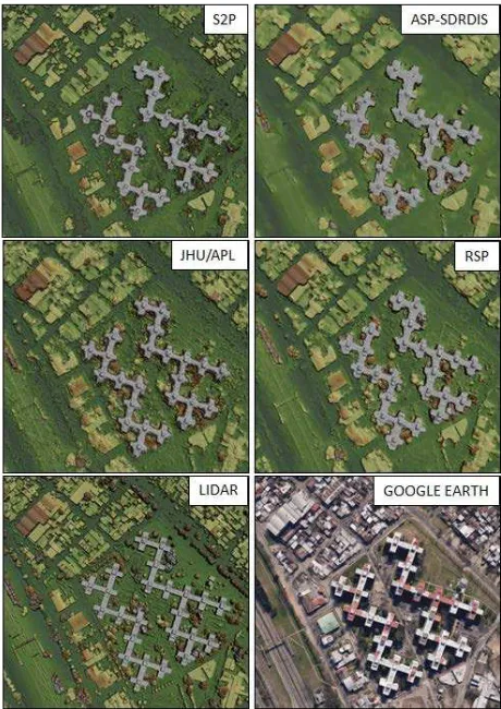
Winning solutions from the contest were based on the Satellite Stereo Pipeline (S2P) (de Franchis et al. 2014), the RPC Stereo Processor (RSP) (Qin 2016), and the NASA Ames Stereo Pipeline (ASP) (Shean et al. 2016). The highest ranking solutions are listed on the MVS3DM Benchmark (2017) web page along with links for open source software downloads for the ASP and S2P solutions and a link for more information about the RSP solution and its use for research purposes. Each of these solutions employed variations of the Semi-Global Matching (SGM) method of Hirschmuller (2008). The Johns Hopkins Applied Physics Laboratory (JHU/APL) also developed an example MVS solution based on the SIFT Flow method of Liu et al. (2011) for comparison. For our current analysis, we consider point clouds produced by S2P, RSP, JHU/APL, and Sebastian Drouyer’s solution based on ASP (ASP-SDRDIS) for one of the test areas from the contest which includes a range of urban structures, as shown in Figure 2.
Figure 2 MVS and lidar point clouds are rendered as digital surface models and compared with Google Earth imagery.
3. GROUND TRUTH PIPELINE
We have begun development of a semi-automated ground truth pipeline designed to quickly generate building footprints over large areas where known building polygons do not already exist. The pipeline currently makes use of high-resolution 3D lidar data for automated labeling of buildings and a high resolution orthorectified image to facilitate manual review and refinement of building polygons.
The area shown in Figure 2 and used in section 4 to demonstrate our metric analysis pipeline covers approximately 0.3 square kilometers. However, we intend to eventually perform analyses over much larger areas, so the proposed ground truth development methods are intended to scale gracefully to hundreds of square kilometers, though there is work remaining to be done to enable that capability.
3.1 Automated Semantic Labeling
We first produce minimum and maximum height images from a dense lidar point cloud, and subsequent filtering, segmentation, and classification steps are performed on those images. Since multiple-return lidar reports ground heights as well as canopy heights over foliage and other vegetation, we first classify vegetation using the minimum and maximum height images. We then extract candidate building boundary edges using gradients in the minimum image, group any connected edges into candidate objects, fill and label those objects, and finally remove small objects to produce a ground-level Digital Terrain Model (DTM) and a raster image indicating ground, building, vegetation, and unknown. Processing 14 million lidar points for the area shown in Figure 2 took approximately 15 seconds on a laptop PC. Processing a larger data set with 600 million points completed successfully in 25 minutes on the same laptop PC with 32 GB of RAM. This scales sufficiently well to enable approximate ground truth production on the order of hundreds of square kilometers without the need for tiling.
Figure 3 shows the building labels produced by our automated method compared with those produced using Global Mapper and LAStools. Ground truth labels produced with the manual editing process to be discussed in section 3.2 are also shown. While all of these results include errors, our automated method produces labels as accurately as the best available alternative.
Figure 3 Automated lidar building classification results from open source JHU/APL software compare favorably to well-established methods.
Additional post-processing is applied to the building label raster image to remove any remaining small objects, produce building footprint polygons, and simplify those polygons to remove unnecessary vertices. Finally, a binary confidence image is produced to indicate pixels for which the building label cannot be determined with certainty. This is not currently used in our analysis, but we expect it to be useful for scaling to larger areas for which detailed manual editing may not be practical. Those pixels would then not be included in accuracy assessment.
3.2 Manual Editing
The second step in our ground truth process is manual review of building footprint polygons and editing to correct any obvious mistakes. We initially used ArcGIS for this. While that application worked well, it quickly became clear that a custom interface designed specifically for our task would be simpler and more efficient, so we developed a MATLAB tool for that purpose.
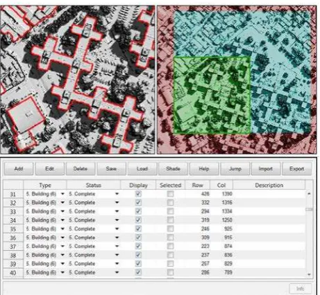
Figure 4 JHU/APL manual editing tool for building polygons includes a drawing window (top left), a context window (top right), and a polygon attribute table (bottom).
Figure 4 shows our manual review and editing tool for building footprint polygons. The top-left window displays a zoomed in view of an orthorectified image and the building outline polygons. Polygons and vertices can easily be created, deleted, or edited using keyboard shortcuts, mouse-enabled menus, and buttons that appear in the center of the figure. Each polygon can be individually labeled with a category from a customizable list. The keyboard is used to navigate around the larger image which is shown in the top-right window, and in the top-left window the user can zoom in for increased detail and out for context. The top-right context window is color coded to indicate which portions of the image have already been viewed. The bottom window shows an attribute table for the building polygons, including category label, review status, polygon bounds, and any user notes.
amount of time without extensive manual effort or online crowd sourcing such as Amazon’s Mechanical Turk. Still, we believe the confidence mask concept discussed in section 3.1 will be important for scaling up to hundreds of square kilometers.
4. METRIC ANALYSIS PIPELINE
The metric analysis pipeline currently assesses 3D point clouds, dense Digital Surface Model (DSM) meshes derived from those point clouds using the maximum Z values, and raster images with semantic labels indicating the locations of buildings. This pipeline will eventually be revised to assess individual 3D building models including facades as well as other static structures in urban scenes. The data considered here does not include those features.
4.1 MVS Point Clouds for Initial Analysis
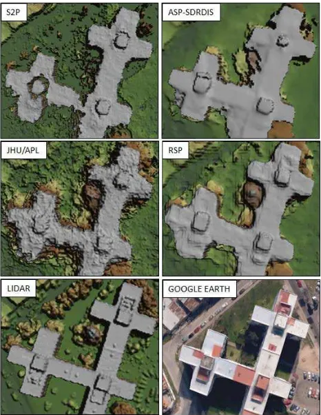
For demonstrating the metric analysis pipeline, we produce 3D point clouds using the four MVS solutions discussed in section 3.2. For each, we use the recommended parameters and the ten image pairs selected by the winning S2P solution from the IARPA Multi-View Stereo 3D Mapping challenge. Figure 5 shows a close up view of a tall housing complex from the same dataset as shown in Figure 2. Visual inspection of the MVS solutions at this scale provides insight into the strengths and weaknesses of each of the solutions which the metrics should capture. For instance, the example solution developed by JHU/APL which does not employ SGM constraints has significantly more Z noise than the other solutions. The S2P solution includes a method to replace rejected unreliable points or data voids with ground height which introduces artifacts with large Z errors on some roof tops. This also replaces many of the trees near the buildings with ground height which results in a clearer separation of some buildings from background for segmentation. Finally, some of the roof tops are visibly dilated in the ASP-SDRDIS and RSP solutions which reduces horizontal mensuration accuracy. These visual observations also manifest in metrics discussed below.
4.2 3D Point Cloud Registration
Before metric evaluation, each MVS point cloud is registered to the lidar ground truth data using a coarse-to-fine search to determine X, Y, and Z translation offsets. These offsets can provide an indication of absolute accuracy when measured in aggregate, but since our analysis is limited to a small localized area, we do not report anecdotal estimates of absolute accuracy.
4.3 MVS Accuracy and Completeness
We begin with the 3D point cloud metrics reported in Bosch et al. (2016) for assessing point clouds submitted for the IARPA Multi-View Stereo 3D Mapping challenge. Median Z error and Root Mean Squared Error (RMSE) are reported compared to a lidar ground truth DSM. Completeness is reported as the percentage of points in the MVS point cloud with less than 1m Z error compared to ground truth. Results are presented in Table 1. Observe that JHU/APL median Z error is significantly larger than the others, consistent with visual inspection in Figure 5. Also observe that the Z RMSE for S2P is larger than the others due to the large Z outliers caused by both trees and small portions of buildings being replaced with ground height. However, S2P also achieves the highest completeness metric which is consistent with overall visual inspection compared to lidar in Figure 2.
Figure 5 MVS and lidar point clouds are rendered as digital surface models and compared with Google Earth imagery. This close up view clearly shows some of the strengths and weaknesses of each of the MVS solutions.
Table 1 Stereo accuracy and completeness metrics for MVS solutions (completeness threshold is 1m)
Metric S2P JHU/APL ASP
4.4 Relative Horizontal Accuracy
The accuracy and completeness metrics commonly used for assessing stereo methods are easy to compute reliably and provide a high level automated assessment of 3D data quality that roughly agrees with visual inspection. However, these metrics conflate all sources of error and generally do not provide a good indication of relative accuracy. Directly measuring relative horizontal accuracy requires a priori knowledge of known scene features. In our pipeline, we employ vector products of buildings to assess relative horizontal accuracy. These vector products may be obtained from public sources such as Open Street Maps (OSM) or derived from lidar using the labeling algorithm described in section 3. OSM vector products require further registration while lidar derived vector products do not since the point clouds are already registered to lidar as discussed in section 4.1.
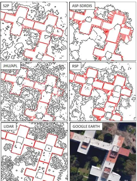
further filtered to form an edge image for comparison with building polygons sampled at the DSM Ground Sample Distance (GSD). Each sampled point from a building polygon is matched with its nearest edge point in the DSM edge image as shown in Figure 6. To account for any residual misalignment, this process is repeated iteratively for each building and the building polygon is translated to minimize the average absolute distance. The horizontal Root Mean Squared Error (RMSE) is then computed for the remaining nearest distances for all building polygons in a scene. Relative horizontal accuracies for lidar and MVS solutions are shown in Table 2. Observe again that roof tops in the ASP-SDRDIS and RSP solutions extend well beyond their true extents. This is clearly indicated in the relative horizontal accuracy metric.
Figure 6 Horizontal accuracy is determined by measuring distances between sampled points on building polygons and nearest edge points.
Table 2 Relative accuracy measured for lidar and MVS
Metric Lidar JHU APL
ASP
SDRDIS S2P RSP
Horizontal
RMSE (m) 0.38 0.80 2.36 1.11 1.73
4.5 Semantic Labeling Metrics
To begin to assess 3D modeling of buildings in urban scenes, we employ common metrics to evaluate 2D semantic labels indicating the presence of buildings in a scene, as summarized in Table 3. Ground truth semantic labels are derived from lidar as described in section 3. The MVS solutions used to initially
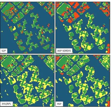
demonstrate the metric evaluation pipeline do not include semantic labels, so we derived building labels with the same algorithm used for lidar. While this is not expected to work especially well, the results shown in Table 4 and Figure 7 offer insight into the challenges associated with labeling MVS point clouds of differing levels of fidelity. Interestingly, even the simple point cloud classification algorithm that only considers geometry produces reasonable labels for the S2P point cloud which has clearly defined building edges for this test data set and which does not include many of the trees. Consideration of additional cues from the image bands along with geometry would better enable separation of manmade structures from nearby foliage and improve the labeling performance for all of the MVS point clouds. Labeling results shown are not intended to indicate the utility of any particular MVS algorithm for this purpose, since those cues have not been considered.
Table 3 Semantic labeling metrics (TP = True Positive, FN = False Negative, FP = False Positive)
Metric Definition Goal
Recall /
Completeness TP/(TP+FN) Higher
Precision /
Correctness TP/(TP+FP) Higher
F Score TP/(TP+0.5(FN+FP)) Higher
Jaccard Index TP/(TP+(FN+FP)) Higher
Branching Factor FP/TP Lower
Miss Factor FN/TP Lower
Table 4 2D building labeling metrics for MVS solutions
Metric S2P JHU/APL ASP
SDRDIS RSP
Completeness 0.79 0.93 0.65 0.91
Correctness 0.86 0.60 0.66 0.60
F Score 0.82 0.72 0.66 0.73
Jaccard Index 0.70 0.57 0.49 0.57
Branching
Factor 0.17 0.68 0.51 0.66
Miss Factor 0.27 0.07 0.53 0.10
4.6 Volumetric Accuracy
Figure 7 2D building labeling accuracy is shown for MVS point clouds (Green=TP, Yellow=FP, Red=FN, and Blue=TN).
Table 5 3D building volumetric accuracy for MVS solutions
Metric S2P JHU/APL ASP
SDRDIS RSP
Completeness 0.82 0.92 0.83 0.93
Correctness 0.84 0.63 0.67 0.61
F Score 0.83 0.75 0.74 0.74
Jaccard Index 0.71 0.60 0.59 0.58 Branching
Factor 0.19 0.59 0.49 0.64
Miss Factor 0.21 0.09 0.21 0.08
Figure 8 3D building height accuracy is shown for labeled MVS point clouds (height color scale is shown in meters).
4.7 Curvature and Roughness Metrics
The perceptual quality of a 3D model depends not only on positional accuracy but also fidelity of shape. Even small inaccuracies in position can have a noticeable effect on the appearance of a model when rendered with direct lighting or a texture map. Lavoue et al. (2013) have assessed computational measures of curvature and roughness similarity and reported that mean curvature and geometric Laplacian metrics correlate well with visual perception metrics. We have implemented the same measures in our pipeline and observed a similar agreement between these two metrics and visual inspection of surface smoothness, as shown in Table 6. These metrics may offer an indication of perceptual quality. Observe the elevated values for S2P due to void fill and for JHU/APL due to excessive Z noise.
4.8 Model Simplicity
Dense 3D meshes are impractical for real-time rendering and transmission over limited bandwidth communications channels. Practical 3D modeling methods reduce geometric complexity by simplifying a dense mesh to reduce triangle count while attempting to preserve accuracy. We measure a model’s triangle simplicity as the fraction of triangles in a 3D mesh of a scene or object and the number of triangles in a mesh sampled at the source imagery pixel Ground Sample Distance (GSD). Similarly, this measure can be generalized to assess geon simplicity for Constructive Solid Geometry (CSG) methods, though we have not yet begun to assess those. The current pipeline assesses simplified triangulated meshes using a subdivision algorithm for direct comparison with a dense ground truth mesh.
Table 6 Curvature and roughness difference metrics compared to lidar for MVS solutions
Metric S2P JHU/APL ASP
SDRDIS RSP Mean
Curvature 0.77 0.67 0.47 0.56
Geometric
Laplacian 0.15 0.12 0.11 0.11
5. DISCUSSION
The ground truth and metric analysis pipelines described here are initial steps toward a comprehensive evaluation capability for 3D modeling of urban scenes based on commercial satellite imagery. The automated labeling software and metric analysis pipeline software have been released for public use with a permissive open source license. For details, please see
http://www.jhuapl.edu/pubgeo.html. We hope that these tools
along with publicly released benchmark datasets will be useful for establishing minimum baselines for expected algorithm and software performance to encourage and enable new research that greatly advances the state of the art. As we continue to refine these tools and apply them to assessing state of the art 3D modeling capabilities, we solicit feedback, criticism, and recommendations from the broad community of researchers for which they are intended.
characterize algorithm performance and provide quantitative indicators of potential defects that may require additional attention, either by an end-user to guide manual editing for 3D model production or by a developer to guide algorithm refinements for producing more consistently accurate results. The MVS solutions released as open source software for the MVS3DM contest offer a unique opportunity for a broad community of researchers to easily begin to experiment with algorithm improvements. We hope that these metric analysis tools can assist in those efforts.
6. FUTURE WORK
The inputs to the current metric analysis pipeline include an MVS point cloud and a raster image indicating building labels. While the point clouds are converted to DSM triangulated meshes for the current analysis, we expect to evaluate more complex 3D scene models in the future. For instance, the Common Data Base (CDB) standard defines a GeoTIFF DTM layer and OpenFlight triangulated mesh building models. Similarly, the CityGML standard defines a DTM and solid and multi-surface building models. As we begin to assess models produced to meet these standards, we will refine the software accordingly.
The 3D metrics in the current pipeline are limited to assessing the 2.5D surfaces readily identifiable in most commercial satellite imagery. When imaged from more oblique viewpoints, either from space or more commonly from airborne sensors, building facades can also be observed sufficiently for 3D reconstruction. We plan to refine our pipeline to include true 3D volumetric assessment compared to high-resolution multi-look airborne lidar (e.g., Roth et al. 2007) and terrestrial lidar (e.g., Nex et al. 2015 and Wang et al. 2016) for assessment of dense 3D reconstruction for complex building facades.
Non-building urban structures such as bridges and complex elevated road networks are not currently included in our metric analysis. This will be addressed in future work as we begin to assess urban areas that include these features.
The metrics defined in this work are also limited to evaluating geometric accuracy only. We are currently also developing ground truth and metric analysis capabilities to also enable assessment of building material classification.
Finally, the current building labeling metrics do not require semantic instance labels for very closely spaced or connected buildings. While it is not at all clear that separate labels and models for those buildings are required or even desirable for many purposes, there are applications for which labeling of individual connected roof structures would be desirable. In future work, we will incorporate instance labels into the ground truth and metric analysis methodologies. We expect these analyses to be targeted to urban areas of very limited size due to the added burden and time of manually editing instance labels.
ACKNOWLEDGEMENTS
The commercial satellite imagery in the public benchmark data set was provided courtesy of DigitalGlobe. The ground truth lidar data was provided courtesy of IARPA. The authors would like to thank Professor Rongjun Qin at Ohio State University for producing the RSP point clouds used for this analysis.
This work was supported by the Intelligence Advanced Research Projects Activity (IARPA) via contract no. 2012-12050800010. The views and conclusions contained herein are those of the authors and should not be interpreted as necessarily representing the official policies or endorsements, either expressed or implied, of IARPA or the U.S. Government.
REFERENCES
Akca, D., Freeman, M., Sargent, I., and Gruen, A., 2010. “Quality Assessment of 3D Building Data,” The Photogrammetric Record, vol. 25, no. 132, pp. 339-355.
Bosch, M., Kurtz Z., Hagstrom S., and Brown M., 2016. “A Multiple View Stereo Benchmark for Satellite Imagery,” Proceedings of the IEEE Applied Imagery Pattern Recognition (AIPR) Workshop.
de Franchis, C., Meinhardt-Llopis, E., Michel, J., Morel, J.-M., and Facciolo, G., 2014. “An automatic and modular stereo pipeline for pushbroom images,” ISPRS Annals.
Campos-Taberner, M., Romero-Soriano, A., Gatta, C., Camps-Valls, G., Lagrange, A., Le Saux, B., Beaupere, A., Boulch, A., Chan-Hon-Tong, A., Herbin, S., Randianarivo, H., Ferecatu, M., Shimoni, M., Moser, G., and Tuia, D., 2016. “Processing of Extremely High-Resolution LiDAR and RGB Data: Outcome of the 2015 IEEE GRSS Data Fusion Contest – Part A: 2-D Contest,” IEEE Journal of Selected Topics in Applied Earth Observations and Remote Sensing, vol. 9, no. 12.
Chen, J., Dowman, I., Li, S., Li, Z., Madden, M., Mills, J., Paparoditis, N., Rottensteiner, F., Sester, M., Toth, C., Trinder, J., and Heipke, C., 2015. “Information from imagery: ISPRS scientific vision and research agenda,” ISPRS Journal of Photogrammetry and Remote Sensing, 115, pp. 3-21.
Hirschmuller, H., 2008. “Stereo processing by semi-global matching and mutual information,” IEEE Transactions on Pattern Analysis and Machine Intelligence, vol. 30, no. 2, pp. 328–341.
Isenburg, M., 2016. “LAStools - efficient LiDAR processing software” (unlicensed version), obtained October 2016 from
http://rapidlasso.com/LAStools.
Koch, T., d'Angelo, P., Kurz, F., Fraundorfer, F., Reinartz, P., Korner, M., 2016. “The TUM-DLR Multimodal Earth Observation Evaluation Benchmark,” Proceedings of the IEEE Conference on Computer Vision and Pattern Recognition Workshops, pp. 19-26.
Lavoue, G., Cheng. I., and Basu, A., 2013. “Perceptual Quality Metrics for 3D Meshes: Towards an Optimal Multi-Attribute Computational Model,” IEEE International Conference on Systems, Man, and Cybernetics.
Liu, C., Yuen, J., and Torralba, A., 2011. “SIFT Flow: Dense Correspondence across Scenes and its Applications,” IEEE Transactions on Pattern Analysis and Machine Intelligence, vol. 33, no. 5.
MVS3DM Benchmark, 2017. Retrieved March 2017 from
http://www.jhuapl.edu/satellite-benchmark.html.
Nex, F., Gerke, M., Remondino, F., Przybilla, H.-J., Baumker, M., Zurhorst, A., 2015, “ISPRS Benchmark for Multi-Platform Photogrammetry,” ISPRS Annals III-1.
OGC Standards and Supporting Documents, 2017. Retrieved 21 March from http://www.opengeospatial.org/standards.
Qin, R., 2016. “RPC Stereo Processor (RSP) – A software package for digital surface model and orthophoto generation from satellite stereo imagery,” ISPRS Annals III-1.
Roth, M., Hunnell, J., Murphy, K., and Scheck, A., 2007. “High-Resolution Foliage Penetration with Gimbaled Lidar,” SPIE Laser Radar Technology and Applications XII.
Rottensteiner, F., Sohn, G., Gerke, M., Wegner, J. D., Breitkopf, U., and Jung, J., 2014. “Results of the ISPRS benchmark on urban object detection and 3D building reconstruction,” ISPRS Journal of Photogrammetry and Remote Sensing, vol. 93, pp. 256-271.
Sampath, A., Heidemann, H. K., Stensaas, G. L., and Christopherson, J. B., 2014. “ASPRS Research on Quantifying the Geometric Quality of Lidar Data,” Photogrammetric Engineering and Remote Sensing.
Shean, D. E., Alexandrov, O., Moratto, Z., Smith, B. E., Joughin, I. R., Porter, C. C., Morin, P. J., 2016. “An automated, open-source pipeline for mass production of digital elevation models (DEMs) from very high-resolution commercial stereo satellite imagery,” ISPRS Journal of Photogrammetry and Remote Sensing, vol. 116, pp. 101-117.
Seitz, S., Curless, B., Diebel, J., Scharstein, D., and Szeliski, R., 2006. “A comparison and evaluation of multi-view stereo reconstruction algorithms,” IEEE Conference on Computer Vision and Pattern Recognition, vol. 1, pp. 519–526.