ASSESSING LANDSAT FRACTIONAL GROUND-COVER TIME SERIES ACROSS
AUSTRALIA’S ARID RANGELANDS: SEPARATING GRAZING IMPACTS FROM
CLIMATE VARIABILITY
J. Barnetson1, S. Phinn1, P. Scarth1, R. Denham2
1University of Queensland, Remote Sensing Research Centre, Queensland, Australia - (j.barnetson, s.phinn, p.scarth)@edu.au 2
Queensland Department of Science, Information Technology and Innovation - [email protected]
KEY WORDS:Fractional ground cover, Non-photosynthetic vegetation, Landsat, Standardised precipitation index, Episodic rainfall, Landsat, Time series, Growth-cycles
ABSTRACT:
Suitable measures of grazing impacts on ground cover, that enable separation of the effects of climatic variations, are needed to inform land managers and policy makers across the arid rangelands of Australia. This work developed and tested a time-series, change-point detection method for application to time series of vegetation fractional cover derived from Landsat data to identify irregular and episodic ground-cover growth cycles. Utilising the High Performance Computing power of the Google Cloud Compute Engine these cycles were segmented to distinguish grazing impacts from that of climate variability. A measure of grazing impact was developed using a multivariate technique to quantify the rate and degree of ground cover change. The method was successful in detecting both long term and short term growth cycles. Growth cycle detection was assessed against rainfall surplus measures indicating a relationship with high rainfall periods. During periods of ground cover decline, grazing utilisation was observed across four major grasslands. Ground cover change associated with grazing impacts was also assessed against field measurements of ground cover indicating a relationship between both field and remotely sensed ground cover. Cause and effects between grazing practices and ground cover resilience can now be explored in isolation to climatic drivers. This is important to the long term balance between ground cover utilisation and overall landscape function and resilience.
1. INTRODUCTION 1.1 Research problem
The aim of this research is to distinguish grazing related ground cover utilisation from that of episodic climate variations in low-photosynthetic arid adapted vegetation. A background to Aus-tralia’s arid rangelands including an understanding of ground cover change and its monitoring, as it relates to ground cover util-isation from grazing related impacts, is first discussed. Next, past and present remote sensing techniques used to distinguish ground cover change from climate response are explained including their limitations and historical development in less arid climates. A time-series approach is next presented that aims to adapt exist-ing techniques and utilise recent advancements in both remotely sensed ground cover imagery, data availability and algorithm de-velopment.
1.2 Understanding change in Australia’s arid rangelands An understanding of change in Australia’s arid rangelands has evolved from early concepts of equilibrium continuum in land-scape system modelling. A system functioning in an equilib-rium continuum is described by (Westoby et al., 1989) as its trend along a path of deterministic succession. This path of determinis-tic succession is argued by others to rarely exist in arid rangelands (Friedel et al., 2000). Unlike a path of succession, landscape pro-cesses in the arid rangelands have been described as a discrete set of ”states” that change or transition from one to another. State and transition changes, described as non-continuous and irreversible, have been observed as a result of management practice. These non-continuous changes are not easily explained by succession or continuous based modelling (Friedel et al., 2000). State and
transition modelling however explains change through the con-cept of resilience. Resilience as described by (Pickup and Chew-ings, 1994) is a measure of the persistence of a system and its ability to absorb change and disturbance. The degree and direc-tion of the resilience of a system through time can be described as its trend. Trend in an arid rangeland system is influenced by both management practices and environmental fluctuations. Separat-ing one from the other is a significant challenge. These foun-dation concepts of state and transition, resilience through per-sistence, trends in management and environmental fluctuations are well researched and embedded in the literature (Friedel et al., 2000, Pickup et al., 1998, Pickup and Bastin, 1997). The chal-lenges they present and the potential uses of remote sensing is discussed further.
1.3 Monitoring change; its complexities, recent advance-ments and opportunities
et al., 2000). Advances in remotely sensed data availability and methods are challenging these historical problems (Hostert et al., 2015, Kennedy et al., 2014). Key breakthroughs include: the unlocking of the USGS Landsat imagery holdings, dense time series are now no longer the domain of coarse and broad scale sensors (Hostert et al., 2015); development and proliferation of high performance computing facilities and algorithm develop-ment (Van Den Bergh et al., 2012), reducing exhaustive and in-tensive processing and; better methods to predict ground cover components, through spectral un-mixing techniques (Hostert et al., 2003, Roberts et al., 2015, Scarth et al., 2010, Schmidt and Scarth, 2009). The opportunity to explore the dynamics of ground cover change as it relates directly to management practices is a practical possibility. Improvements in management practices can be made with an improved understanding of landscape change and its resilience to change (Pickup and Chewings, 1994).
1.4 A time series approach
Existing time series vegetation change detection methods have been developed in more regular seasonally driven climates in-cluding (Verbesselt et al., 2010, Jonsson and Eklundh, 2002) and (Eklundh, 2015). The TIMESAT method of (Jonsson and Ek-lundh, 2002, EkEk-lundh, 2015) was developed to characterise sea-sonal response of vegetation growth in multi-temporal imagery including AVHRR and MODIS. A smoothed time series is used to extract seasonal growth parameters that are then used to deter-mine vegetation growth metrics. TIMESAT is a useful method for characterising the overall pattern or shape of a regular sea-sonally driven time series. Arid vegetation climate responses are more irregular and difficult to characterise. The BFAST or Breaks For Additive Seasonal and Trend method de-constructs a time se-ries into seasonal phenological, overall trend and remainder com-ponents (Verbesselt et al., 2010). Unlike the TIMESAT method that is focused on the growing component of the time series the BFAST method exploits the full temporal detail of the time se-ries. Growth patterns and seasonal shapes in the temporal detail are assessed to detect both abrupt or stepped changes and gradual or gentle linear trends. A decomposition model is used to fit a piece-wise linear trend and seasonal model. An iterative process is next undertaken to detect change or breakpoints in the time se-ries. Breakpoints are easiest to detect where noise levels are low and seasonal amplitude high. (Verbesselt et al., 2010) reported that measurable seasonal amplitude was not apparent in NDVI imagery in arid and frozen areas. This type of seasonal pheno-logical modelling in arid environments is problematic. A gap ex-ists in availability of suitable measures and methods for arid and irregular climate driven environments. Development of specific methods and appropriate remotely sensed data is needed. Further to this, the inability to separate climatic drivers from land man-agement practices is due in part to the limitations in available im-agery and the dominance of inappropriate indices and time-series approaches (Friedel et al., 2000). Many studies, including (Evans and Geerken, 2004a), have been limited to annual / biannual im-agery or course resolution imim-agery at more regular temporal in-tervals.
1.5 Research objectives
The main objective of this research is to develop new and expand existing methods to differentiate and measure grazing impacts on ground cover from that of climatic variability in remotely sensed Landsat Fractional Ground Cover (LFGC) time series data. Utilising advancements in spectral un-mixing methods used in the development of the LFGC data by (Scarth et al., 2010) and
(Schmidt and Scarth, 2009), improved estimates of actual ground cover information vs. indices of ground cover, at an appropriate temporal and spatial scale, is now accessible and able to be efficiently processed in a dense time series manner, to further understand differences in ground cover change induced by management and climate. To do so this research first developed and tested an automated method to identify irregular growth cycles in LFGC time series data with the aim to identify and attribute the most distinguishable periods of livestock pasture utilisation. The rate and degree of ground cover decline within each utilisation period providing a measure of climate adjusted management impact.
Irregular or episodic ground cover growth cycle detection involved the development of an adapted time-series change-point detection method. LFGC remotely sensed imagery developed by (Scarth et al., 2010) and (Schmidt and Scarth, 2009) models the fractional proportions of ground cover as: green or pho-tosynthetic vegetative (PV) cover; dead or non-phopho-tosynthetic vegetative (NPV) cover; and bare earth non vegetative cover; from field measured observations. Illustrated in figure 1 each fraction differs from one another throughout their growth cycles. Any attempt to decouple climate from management effects in LFGC should investigate such differences. The two major growth cycles of 2001 and 2010 illustrated are an example of these differences. Beginning with the growth of vegetation cover in response to rainfall, the NPV or dry / low photosynthetic fraction is observed to be significantly higher than that of the PV response. This is both a process of growth, senescence and accumulation of dry plant material and a dominance of the vegetation fraction. The later a result of plant adaptations of arid / semi-arid plant species that aim to lower photosynthesis and transpiration rates, to conserve water (Tomlinson et al., 2013). The first change point is identified as the upper growth point or peak of the NPV response. Illustrated in figure 1 this is the point whereby climate driven growth has ceased and decline is observed to follow. The trough is the other change point whereby either ground cover vegetation is observed to have been completely removed and / or climate begins to influence growth once again. The derivative of a statistical model was used to identify these change or break points in NPV ground cover growth. Time series segmentation was then used to classify NPV ground cover growth cycles between each peak and decline break point. These cycles were further segmented to distinguish grazing impacts from that of climate variability. Grazing impact was measured to quantify the rate and degree of ground cover change. The method detected long and short term growth cycles. Growth cycle peak detection was assessed against rainfall surplus measures indicating a relationship with high rainfall periods. During periods of ground cover decline grazing utilisation became evident. Change associated with grazing impacts was assessed against field measurements of ground cover indicating a relationship between field and remotely sensed ground cover.
2. MATERIALS AND METHODS 2.1 Study area
Figure 1. Landsat Fractional Ground Cover time-series plot of a one hectare area of arid rangeland. Major change points indicate ground cover growth cycles. The NPV growth cycle is notably
larger than the PV.
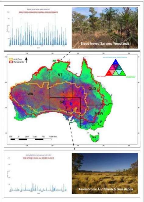
illustrated by the green photosynthetic component of the Landsat fractional ground cover product in figure 2. The other is the arid zone, defined by the K¨oppen-Geiger climate classification (Peel et al., 2007), rainfall is low and episodic. The vegetation is a mix-ture of xeromorphic arid shrub-lands and grasslands with lower levels of photosynthetic material. The study area is focused on these arid rangelands. It is a largely intact natural landscape of approximately 3 millionkm2. Less than 5% has been cleared for
agriculture, horticulture or urbanisation (and Sciences and Eco-nomics, 2016) and mining, tourism and livestock production are the main economic activities. Rangeland grazing for beef and sheep production is the most extensive, encompassing approx-imately 50% of the area (and Sciences and Economics, 2016). Two extensive land tenures exist: freehold Aboriginal land used primarily for traditional living and some rangeland grazing; and freehold and leasehold pastoral lands utilised primarily for range-land grazing (and Sciences and Economics, 2016). Rangerange-land grazing utilises native and introduced pastures in a natural sys-tem for animal production.
2.2 Landsat Fractional Ground Cover Data (LFGC) 2.2.1 Suitability LFGC imagery developed by (Scarth et al., 2010) and (Schmidt and Scarth, 2009) is used in this study for a number of reasons. First Landsat being the longest archive of re-motely sensed earth surface observations in the world (Kennedy et al., 2014) and spanning several decades it is most suited in detecting irregular and episodic vegetation change in an arid en-vironment. Moderate spatial resolution multi-spectral image data will continue to be collected globally by several nations and is the most widely used source of environmental monitoring data. Next it provides the necessary spatial resolution to depict management related change. (Roy et al., 2015) and (Bastin et al., 1995) suggest a spatial scale or grain of one hectare is important to most land-scape scale processes and monitoring programs in rangelands. Lastly and importantly the LFGC imagery aims to model the frac-tions of ground cover of a remotely sensed image pixel from field based observations. These fractions include photosynthetic veg-etative (PV) cover, dead or non-photosynthetic vegveg-etative (NPV) cover, and bare earth non vegetative cover including rock and stone. (Scarth et al., 2010) developed a constrained un-mixing al-gorithm to estimate these fractions in Landsat imagery from field based training data. Each fraction is represented by the three pri-mary colours illustrated in the colour triangle in figure 3 along with corresponding field photographs. An example LFGC im-age of Australia in figure 2 next illustrates each fractions colour
BARE MIX
PV MIX NPV MIX NPV & BARE
NPV & PV NPV
BARE & PV
BARE PV
NON-PHOTOSYNTHETIC VEGETATION (NPV)
BARE GROUND PHOTOSYNTHETIC
VEGETATION (PV)
Broad-leaved Savanna Woodlands
Xeromorphic Arid Shrub & Grasslands
Figure 2. Extent of the Australian rangelands and its arid zone. Differences in climate and vegetation can be seen between the northern equatorial Savannah’s and the dry episodic arid shrub-lands and grasslands.
representation. Arid vegetation has adapted to reduce water loss through reducing respiration and photosynthesis (Tomlinson et al., 2013). (Pickup et al., 1994) reported that traditional methods are limited in their ability to separate less photosynthetic vegeta-tion from that of background soil. This low or non-photosynthetic cover (NPV) component of vegetation cover is dominant in arid landscapes, as further illustrated in figure 2. LFGC unlike tra-ditional remotely sensed vegetation methods aims to ’un-mix’ or separate both the living and non-photosynthetic vegetation com-ponents from each other and from background earth, rock and stone.
2.2.2 Preprocessing and standardisation LFGC is derived from the US Geological Service (USGS) Landsat 5, 7 and 8 level one terrain corrected holdings. (Flood et al., 2013) and (Flood, 2014) have applied atmospheric, topographic and Bidirectional Reflectance Distribution Function (BRDF) radiometric calibra-tions to the Landsat data to derive surface reflectance imagery. Cloud masking has also been applied using techniques developed by (Goodwin et al., 2013). Single date path-row images in 16 day intervals from 1987 to present will be used in a time series based analyses. The study area is resolved by 192 individual Landsat scenes (see Figure 4) that consists of≈130thousand individual
PHOTOSYNTHETIC VEGETATION (PV)
NON-PHOTOSYNTHETIC VEGETATION (NPV)
BARE MIX
PV MIX NPV MIX NPV & BARE
NPV & PV NPV
BARE & PV
BARE PV
NPV & BARE
BARE MIX
BARE BARE & PV
NPV & PV NPV
PV BARE GROUND
Figure 3. Field photographs of fractional ground cover components and their corresponding colour triangle representation.
Figure 4. Location of fractional ground cover field measurement sites and Landsat imagery extents.
2.2.3 Field estimates of fractional ground cover The 978 field sites in figure 4 were established by various state and terri-tory government agencies, for the purposes of calibrating and val-idating both MODIS and Landsat fractional ground cover prod-ucts (ABARES, 2013). The NT Department of Environment and Natural Resources (DENR) rangelands monitoring branch from 2013 to 2017 established 700 of the 978 field sites for the pur-poses of rangeland monitoring including on-going validation and calibration of the LFGC imagery. Field site stratification and placement involved a desktop assessment of land and vegeta-tion resource mapping and satellite imagery to ensure site homo-geneity and representation. Patches of intact and minimally dis-turbed vegetation, no less than 100 x 100m in size were selected. Following the national standard ground cover field measurement method of (Muir et al., 2011), each site consists of 300 individual point intercept observer estimates. Utilising a laser pointer for the ground and mid vegetation layer (<2m above ground level) and a sight tube densitometer for upper canopy vegetation, frac-tional ground cover and projected foliage canopy cover intercepts are observed and recorded at one metre intervals along three star pattern arranged 100m measuring tapes as illustrated in figure 5.
(A) (B)
Figure 5. (A) Example of point intercept field collection method. (B) Star transect alignment of 100m point intercept transects with Landsat 3 x 3 pixel window
2.3 Time-series analysis method
Change point detection in NPV growth cycles is the aim of the first stage of the time-series method. A ”change point” is de-fined as the point in a growth cycle were by a major phenological change has occurred. A growth cycle is defined as having two key components: (1) the response and accumulation of NPV ground cover to rainfall including its peak or maximum growth change point and, (2) its subsequent decline to a point of either complete ground cover removal or response to rainfall again, defined as its trough or minimum change point. Long term growth cycles are defined for the purposes of this study as those generally greater than three years in duration and the result of continued rainfall events. Short term cycles on average are less than three years but more typically one to two years and are likely attributed to annual - biannual rainfall cycles. Characterisation of each growth cycle is the next stage. Ground cover utilisation within each growth cycle is determined and classified, then the amount and rate of decline is assessed. The following describes each stage in detail.
2.3.1 Field site stratification The time-series based method was developed and tested on a stratified sample of the previously described field sites and associated image subsets. The Aus-tralian National Vegetation Information System (NVIS) (Keith and Pellow, 2015) was used to determine dominant and exten-sive vegetation communities, in particular those with a significant grassland structure. The long-term rangeland monitoring photo database, developed and maintained by the Northern Territory Department of Environment and Natural Resources, provided in-formation about pasture utilisation. Both formed the basis of the stratification process.
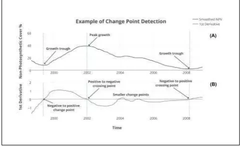
2.3.3 Change point detection The first step in detecting change points in the NPV time series was to smooth the time series in an attempt to remove noise. Efforts have been taken to improve the signal to noise ratio through atmospheric, albedo and terrain corrections applied to the Landsat imagery in the pre-processing stages discussed in the LFGC data section. How-ever soil moisture and its effects on soil brightness, reported by (Pickup et al., 1994), and further atmospheric effects from smoke, dust, haze and light cirrus cloud are additional sources of noise in the LFGC imagery that are difficult to remove at the pre-processing stages. A method of interpolating a spline between individual NPV data points to smooth the time series and remove this noise, whilst still characterising the signal was used. The Python scientific programming module SCIPY was used to im-plement a one-dimensional smoothing spline fitted to each NPV time series. The smoothing spline is a method of fitting a curve to a set of noisy observations using a spline function. The next step was to locate the positions of the change points in the time-series. Defined as points of extremes i.e. maximum growth peaks and minimum troughs, we use a first derivative test to find these max-ima and minmax-ima in the time-series. Differential statistics were used to calculate the first derivative of the spline function used to smooth the time-series. The point in the derivative time series that crosses thexaxis from positive to negative change is illus-trated in plot (B) of figure 6 as the blue line. This is the point whereby growth has reached a local maximum peak and begins to decline as illustrated in the plot (A) of figure 6 as the coinci-dental blue line. The opposite negative to positive crossing point is the extreme minimum position in the derivative time series and is illustrated as the red vertical line in plots (A) & (B) of figure 6.
Figure 6. Example of minimum and maximum NPV change point detection. Plot (A) illustrates a time series of NPV cover, a smoothed spline fitted to the time series and the locations of the peak (blue) and (red) trough change points. Plot (B) is a first derivative time-series of the spline function in the top plot. Thex
crossing axis points illustrated in blue and red are used to determine the locations of the maximum and minimum change points in the top plot.
2.3.4 Change point assessment (Nicholson et al., 1990) re-ported that rainfall is a driver of vegetation response in a range of landscapes and (Evans and Geerken, 2004b) found it to be lin-early correlated to ground cover growth in arid environments. Figure 7 illustrates the relationship between rainfall and low-photosynthetic ground cover in an arid grassland. This relation-ship was used to assess the accuracy of the detection of LFGC growth cycle peaks. The trough of the growth cycle is diffi-cult to assess in this manner. It is proposed, primarily a
func-tion of ground cover utilisafunc-tion and assessed further (see secfunc-tion 2.3.8). Positive rainfall anomalies or peaks in the long term rain-fall record were identified using the Standard Precipitation Index (SPI) of (McKee et al., 1993) and compared to that of the peaks detected in the NPV time series. SPI is a normalised index rep-resenting the probability of occurrence of an observed rainfall amount when compared with the rainfall climatology at a loca-tion over a long-term reference period. Developed by (BOM, 2015) and accessed through an archive established by (Jeffrey et al., 2001) the 5km2 gridded monthly rainfall surfaces were used to calculate SPI time series for the length of the Landsat archive. SPI enables rainfall conditions to be quantified over varying time scales. For example, shorter temporal windows can be used to determine temporary soil moisture changes in agricultural ap-plications whereas longer windows can indicate water storage shortages and droughts. A long temporal analysis window of 36 months was chosen to detect anomalies present in infrequent / episodic rainfall patterns typical across the arid and semi-arid rangelands of the study area. Vegetation responds to rainfall at varying rates depending on factors aside from plant physiology, such as rainfall timing, soil temperature and soil type. A method of calculating the lag between rainfall and NPV growth was em-ployed. A cross correlation technique was used to determine the relationship between NPV cover and SPI for each individ-ual growth cycle in the time-series. Cross correlation is the mea-sure of similarity of two series as a function of the displacement of one relative to the other (Rabiner and Schafer, 1978). This displacement or offset value is calculated indicating the degree of positive or negative lag between the two variables through-out each individual growth cycle. Climate over the longer term contributes to each and every growth cycle, however the aim of this method is to identify the effects of rainfall acting upon each ground cover growth cycle as an assessment of the change point detection method. Figure 8 illustrates an example of an NPV and SPI time series for a particular growth cycle and their offset. The position of the NPV peak in the time series was next adjusted by this offset and the coincidental SPI value extracted at this loca-tion in the time series as the lag adjusted SPI for that NPV peak. Next, each lag adjusted SPI value was classified into the rankings in table 1 that come from the modified classification of (McKee et al., 1993) by (H¨ansel et al., 2016). Positive SPI values above 1 indicate moderate to extremely wet rainfall anomalies and vice versa for negative values less than negative 1 with normal to near normal in the 1 to -1 range. The percentage of positive rainfall SPI peaks from the time series of every field site across the study area provided an indication of the performance of the change de-tection method to detect NPV peak change points.
Table 1. Standardised Precipitation Index classification SPI Start SPI End Category
2 >2 Extremely Wet
1.5 1.99 Very Wet
1.0 1.49 Moderately Wet
-0.99 0.99 Near Normal
-1.0 -1.49 Moderately Dry -1.5 -1.99 Severely Dry
-2 <-2 Extremely Dry
cy-Figure 7. Example of a time-series of non-photosynthetic ground cover (A) in an arid grassland and its corresponding rainfall time-series (B), illustrating the response of ground cover to rainfall.
Figure 8. Example of NPV growth cycle and coincidental SPI time series. The NPV growth peak (black circle) and its lag or offset to the SPI time series (vertical dashed lines) is illustrated. The adjusted SPI value (blue circle) is also demonstrated.
cle based on its duration was then defined as either long or short term. The first stage of each growth cycle was defined as the pe-riod from the initial minimum growth trough to its peak. Titled the growing stage, ground cover including NPV cover increases in response to rainfall. Phenological processes of photosynthe-sis, growth, senescence and accumulation are occurring as are re-moval processes including grazing and decay. The next stage was defined as the period from the peak growth point to the next min-imum trough point. Illustrated as the utilisation stage of a growth cycle in figure 9. Ground cover was observed to have reached a peak in both growth and accumulation. NPV cover begins to de-crease. The effects from management practices such as grazing are considered to be most prominent during this stage and those of climate such as rainfall least prominent. Differences between each individual time series across each image subset with simi-lar climate and vegetation characteristics were used to test this. Climate should mask any management related effects during pe-riods of substantial growth. During pepe-riods of decline, distinction between time-series as a result of differing grazing intensities be-came evident.
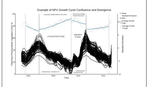
2.3.6 Growth stage confluence and divergence The conflu-ence and divergconflu-ence between each individual pixel time-series across an image subset was used as a method that indicated and illustrated the previously described effects of climate and graz-ing intensity. Illustrated in figure 9 the first step involved the
calculation of the standard deviation between each pixel time se-ries across an image subset. Next a method of determining a single date that represented the major growth peak and trough lo-cations, previously determined, across all of the individual pixel time-series was developed and the major growth cycles of each image subset identified. A linear model was next fitted to the standard deviation time-series between each growing and utilisa-tion stage of each major growth cycle. During the growing stage of each cycle the slope of the model was tested for a negative trend, indicating a confluence of each NPV time series that in-dicated a masking of the effects of differing grazing intensities across the image subset. During the utilisation stage the slope of the model was tested for a positive trend, indicating a divergence of each NPV time series from one another and highlighting dif-ferences in grazing intensities. This was carried out across the four stratified grassland image subsets.
Figure 9. Example of a number of NPV growth cycles across an image subset, their utilisation and growth stages and the divergence and confluence between them as a function of grazing intensity and climate response.
2.3.7 Rate and degree of NPV utilisation The decline in NPV ground cover during the utilisation stage of the growth cy-cle were measured in terms of their amount and intensity. The rate of which it declines gave an insight into the intensity of the removal process. First a linear model was fitted to each utilisa-tion segment from its peak growth point to its proceeding trough and the models slope used to determine the rate of which NPV ground cover declined for each utilisation stage. The amount of the decline provided a measure of the degree of both the spatial extent and amount of cover removed by grazing practices. Factors that complicate this included the distinction between palatable and unpalatable vegetation including woody vegetation and the distinction between detached plant material as litter and standing senescent plant material. Adapted from (Jonsson and Eklundh, 2002) and defined in figure 10 two measures were developed to begin to understand these differences. Both quantified the amount of cover decline as an approximation of the area under each util-isation segments curve. The larger area or integral encompassed the entire area under each utilisation curve, defined by the verti-cal axes of the peak and trough locations, the curve of the fitted spline and the horizontal base of zero cover. The smaller area / integral differed in that the horizontal base was defined by the trough point location. Differences between them provide insights into the challenges presented.
Figure 10. Example of the utilisation period of a growth cycle. Defined as the point from the growth peak to the proceeding trough, measures of both the rate and degree of utilisation are illustrated as a linear model of slope from the peak to the trough and the area under the curve. The large area under the curve integral has anxaxis base of zero and the smaller integral an adjusted base at theytrough point.
the performance of the growth cycle characterisation and sub-sequent utilisation segmentation to accurately define periods of decreasing NPV fractional cover. Each segment was tested for a downward monotonic trend using the Mann-Kendall test devel-oped by (Kendall, n.d.). Each pixel time-series within an image subset chip was tested for each of the stratified grassland image subsets. The presence of a decreasing trend and the significance of the trend was then reported.
3. RESULTS 3.1 Field site comparisons
Figure 11 illustrates the relationship of field measured NPV with the LFGC derived NPV. On theyaxis is the coincidentally ac-quired LFGC NPV fraction and on thexis the measured field NPV fraction. The residual error and bias are also indicated.
Figure 11. Field site measured NPV compared with coincident date LFGC derived NPV
3.2 Time series analysis
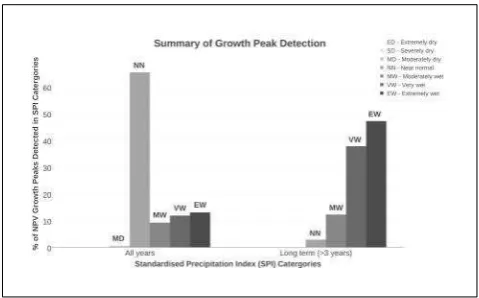
3.2.1 Change point detection Figure 12 illustrates the pro-portion of NPV growth peaks that were associated with each standardised precipitation index classification class. NPV growth peaks associated with long term growth cycles show the strongest
relationship with all of the peaks detected in near normal to ex-tremely wet conditions. The remainder shorter term peaks are associated with near normal conditions for the majority with a very small (5.6%) detected in moderately dry conditions across the 568 field site time series.
Figure 12. Results of NPV growth peak assessment. All Peaks were assessed in the series on the left of the chart and only the peaks associated with long term growth cycles were assessed in the series on the right. In both series less than 6% of the growth peaks were detected in periods of moderately negative SPI.
3.2.2 Growth cycle characterisation The locations of the four example field sites and their time-series plots are illustrated in figure 13. Field site (A) is located in a sub-tropical to semi-arid Eucalyptus low-open woodland / tussock grassland, in the north-ern region of the study area. These grasslands are extensively grazed yet not expansive across the arid zone. Field site (B) is located in a mixed chenopod shrub-land / grassland. These grass-lands are also extensively grazed and are moderately expansive across the arid zone, particularly throughout southern parts of the Northern Territory and northern parts of South Australia. Field site (C) is located in an introduced Buffel (Cenchrus ciliaris) pas-ture grassland / low-open Eucalyptus woodland. Mostly associ-ated with the alluvial plains and channels of the inland rivers and drainage systems, they are also extensively grazed. The last field site (D) is located in a Spinifex (Triodia sp.) hummock grassland. Infrequently grazed it is however the most expansive grassland of the study area. A sequence of historical field-based site photos illustrate changing ground cover utilisation both in the photo and the time-series. Lastly a high resolution true colour satellite im-age provides spatial context of each associated NPV imim-age subset extent and its general landscape characteristics.
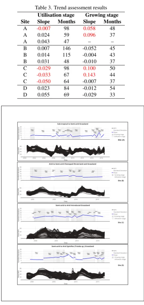
3.2.3 Growth cycle confluence and divergence The conflu-ence and divergconflu-ence of the individual time-series of the four grassland examples is illustrated in figure 14. A time-series of the standard deviation between each of the NPV time-series at each example subset is illustrated. The slope of the standard de-viation of each generalised cycle is further illustrated as a blue line, indicating either a positive upward trending slope, as a con-fluence of the time-series, or as a negative downward trending slope, as a divergence of the time-series. The slope of each stage and its trend is further summarised in table 3 for each sites major (>3 years) growth and utilisation stages.
SITE (A)
PLATE 1. JULY 2000 PLATE 2. OCT 2004 PLATE 3. MAY 2015
PLATE 1
PLATE 2 PLATE 3
PLATE 2. JUNE 2007 PLATE 3. OCT 2012 PLATE 1. MARCH 2004
PLATE 1 PLATE 2
PLATE 3
PLATE 1. OCT 2013 PLATE 2. JUNE 2007 PLATE 3. OCT 2012 PLATE 1. MARCH 2004
PLATE 1
PLATE 2
PLATE 3
PLATE 1 SITE (B)
SITE (C)
SITE (D)
Figure 13. Field site time-series plots of the four example. Each plot illustrates each sites growth cycles, associated growth peaks and troughs, field site visit photos and the extent of each image subset.
integrals encompassing the area from each cycles minimum de-cline point horizontally to its peak and the larger integrals from each plots zero base. The slope of each segment from its peak to its trough is shown as a dark line illustrating the rate of NPV decline.
3.2.5 Decreasing trend assessment The monotonic trend as-sessment of each utilisation stage for the centre pixel time-series in each of the example field sites is presented in figure 16. The trend of each individual utilisation stage is illustrated. Each of these stages with the exception of one short term (<3 years) stage in field site (C) showed a downward or negative trend. Each of the time-series in each field site image subset was also assessed and only a very small proportion (<1%) was fond to have no signif-icant downward trend with a confidence level of 98% as detailed in table 2.
Table 2. Monotonic trend assessment results Site Decreasing trend % AverageZ AverageP
A 99.23 -3.217 0.0035
B 99.78 -3.150 0.0038
C 99.64 -3.161 0.0040
D 99.58 -3.194 0.0036
4. DISCUSSION
4.1 Importance of field data calibrated remotely sensed im-agery
As (Guerschman et al., 2015) states,monitoring vegetation con-tinuously across large landscapes requires robust remote sensing
Table 3. Trend assessment results Utilisation stage Growing stage Site Slope Months Slope Months
A -0.007 98 0.058 48
A 0.024 59 0.096 37
A 0.043 47 – –
B 0.007 146 -0.052 45
B 0.014 115 -0.004 43
B 0.031 48 -0.010 37
C -0.029 98 0.100 50
C -0.033 67 0.143 44
C -0.050 64 -0.007 37
D 0.023 84 -0.012 54
D 0.055 69 -0.029 33
Site (A)
Site (D) Site (B)
Site (C)
Figure 14. Confluence and divergence plots of the four example grasslands. The top plot of each site details (1) each generalised growth and utilisation stage highlighted in shades of grey, (2) the time-series of the standard deviation between each NPV time-series and (3) the slope and trend, annotated and indicated by the blue line, of the standard deviation for each stage. The bottom plot of each site details the individual subset fitted NPV time-series.
Site (A)
Site (D) Site (B)
Site (C)
Figure 15. Example field site plots illustrating each sites growth cycle utilisation stage. Measures of utilisation are further illustrated as both the area under the curve and the slope of each stages decline.
LFGC imagery used in this study, in particular the NPV fraction, is an example of a remotely sensed image technique that more accurately depicts ground cover vegetation in arid environments than those used in previous studies (Hobbs, 1995, Holm et al., 2003). Insensitivity to low-photosynthetic material described by (Friedel et al., 2000) has been the primary limitation of past stud-ies and has been demonstrated to have been improved. A limita-tion however is in the ability of the LFGC imagery to accurately model ground cover across a complex range of vegetation types across Australia and in-particular the low photosynthetic environ-ments of the arid zone. An iterative process of model recalibra-tion and product validarecalibra-tion with further field data is required.
4.2 Accurate time-series change point detection
The next stage of the discussion involves the assessment of the detection of change points to distinguish growth cycles in time-series of NPV ground cover. Confidence in the change point de-tection method is key to the distinctions of growth cycles, seg-mentation of utilisation stages and their associated metrics. As a function of the response of ground cover to rainfall, growth peaks were detected and assessed against peaks in rainfall. Figure 12 shows that less than 6% of the NPV growth peaks were not asso-ciated with peaks in normal to wet conditions. Confidence in the method to detect peaks in individual NPV growth cycles has been demonstrated. Influences of longer term climatic drivers remain unknown and should form the basis of further study.
4.3 Irregular growth cycle characterisation
Adapting and building upon the time-series analysis methods of (Verbesselt et al., n.d.) and (Eklundh, 2015), this method demon-strates its potential to detect more irregular and less seasonally
Site (A)
Site (D) Site (B)
Site (C)
Figure 16. Individual pixel NPV time series plots of the four grassland field site image subsets. The monotonic trend of each utilisation stage is illustrated, indicating a majority of negative downward trends for each stage in each time-series.
4.4 Examples of decoupled ground cover utilisation from climate variability.
Management related impacts de-coupled from environmental fluctuations in ground cover is a challenging problem. Previous studies, such as the Dynamic Reference Cover Method (DRCM) of (Bastin et al., 2012) aimed to do so through careful selection of remotely sensed imagery that depicts a period of least climatic influence. Bench mark areas of highest ground cover in the se-lected dry time are identified and compared with the surrounding landscapes as a measure of management related change. Useful in areas of relatively homogeneous vegetation, the complexities of soil and vegetation across the landscapes of central Australia have proven difficult to make meaningful comparisons within the limitations of available landscape stratification resources. The method in this study takes a different approach in that it attempts to identify the segments of each image pixels time-series with the least climatic influence. Vegetation and management related changes are defined across a much longer and more detailed pe-riod than a single dry pepe-riod point in time. The NPV time-series across each of the four example field sites in figure 14 illustrate these dynamic changes in ground cover. Each shows how time-series of similar characteristics both con-flux and diverge from one another throughout their growth cycles. During the initial stages of growth and accumulation of leafy and woody material in response to rainfall, time series converge and potential differ-ences in vegetation characteristics and importantly management related impacts appear least evident. During the utilisation and decline stages of each NPV cycle, previously described as the pe-riod from peak growth to the proceeding growth trough, time se-ries are observed to separate from one another. It is this separation or divergence that provides insight to the ability of the method to identify and distinguish differences in grazing related ground cover change. This is quantified through the assessment of each sites growth stage variability between each individual time-series and the slope of that variability. Table 3 summarises each sites slope for each of the four growth stages per site. The slope of each of these stages at site (A), the sub-tropical to semi-arid grassland, is as expected for two of the three utilisation stages and unex-pected for the two growing stages. Climate in these landscapes is a mixture of arid episodic irregular rainfall and tropical monsoon. The separation of climate from the perceived management effects is difficult in these landscapes. Sites B & D do follow a pattern of confluence of the time-series during the growing stages and divergence during the utilisation stages. Site (C), the introduced grassland does not show strong confluence and divergence trends. This is likely the result of the image subset location encompass-ing a higher degree of grazencompass-ing variability. Figure 13 illustrates the location of a stock watering point, a source of heavy graz-ing. A number of time-series in the bottom plot of figure 9 (site (c)) can seen to decrease rapidly following the first major growth stage suggesting intensive and localised grazing. Each of the four field site plots illustrate a gradual divergence of each time series in some instances and a sudden divergence in others, each likely due to differences in management practices and vegetation char-acteristics and each an important factor when attempting to un-derstand and separate these effects from that of climate response.
4.5 Measures of management related ground cover utilisa-tion
A measure of the degree of management related change is next discussed. Numerous time-series metrics have already been de-veloped. The TIMESAT method of (Eklundh, 2015) utilises a number of metrics including the area under the curve. This along
with a slope based measure of the rate of decline in NPV cover are illustrated in figure 15. The plot of field site (A) shows the slope of each segment’s decline to be relatively steep and the area under the curve moderately variable from segment to segment. Site (B) in contrast is more gradual and the area under each curve has a larger proportion of the smaller integral. Site (C) is sim-ilar to site (A) and site (D) has the least degree of NPV utili-sation. Sites (A,B& C) are intensively grazed and site (D) less so. Site (B) interestingly is the introduced species of grassland and is more resilient to grazing. Useful insights into management related changes are observed. A better understanding of these changes will lead to more effective monitoring of the changes and trends in rangeland state and condition (Friedel et al., 2000, Pickup et al., 1998, Pickup and Bastin, 1997).
4.6 Assessing ground cover utilisation
Scale appropriate historical information about the utilisation of ground cover across the study area that could be applied to LFGC remotely sensed imagery is lacking. A statistical assessment of the methods ability to define the periods described as the utili-sation stage in the absence of this data was undertaken. Each utilisation segment tested true to a monotonic decreasing trend using the Mann-Kendall test with the exception of a very small proportion (<1%). This was was only present in smaller utilisa-tion sample sizes (n<7).
5. CONCLUSIONS AND FURTHER RESEARCH
5.1 Concluding remarks
A method that utilised and adapted existing techniques was de-veloped and applied in a new approach to the decoupling of man-agement related effects from that of climatic variations. Charac-terising irregular ground cover growth cycles utilising dense time series methods is a new approach. Seasonally driven growth cy-cle studies utilising traditional remote sensing image indices are more common. This study demonstrated that an accurate charac-terisation of episodic rainfall driven growth cycles, that utilised a more appropriate measure of ground cover, is possible.
5.2 Ongoing research
ACKNOWLEDGEMENTS
Support from the Australian Government Research Training Pro-gram Scholarship. Support and funding from the University of Queensland Joint Remote Sensing Research Agreement. Support and funding from the NT Department of Environment and Natu-ral Resources / QLD Department of Science, Information Tech-nology and Innovation Collaborative Research Agreement. QLD Department of Science, Information technology and Innovation staff at the Eco-sciences Precinct Remote Sensing Centre for assistance, support, training, advice and access to High Perfor-mance Computing Infrastructure including: John Armston, Lisa Collet, Neil Flood, Rebecca Trevithick, Dan Tindall and Fiona Watson. NT Department of Environment and Natural Resources staff and volunteers for assistance in collecting fractional ground cover field data including Gary Bastin, Peter Brockelhurst, Nick Cuff, Jock Duncan, David Hooper, Megan Humphries, Debbie Mitchell, Andrew Scott, Grant Staben, Laurie Tait, Sarah Thorne and Cameron Wallace.
REFERENCES
ABARES, 2013. Australian ground cover reference sites database. Technical report, Australian Bureau of Agricultural and Resource Economics and Sciences, Canberra, Australia.
and Sciences, A. B. o. A. and Economics, R., 2016. The Aus-tralian Land Use and Management Classification Version 8. Tech-nical report, Australian Bureau of Agricultural and Resource Economics and Sciences, Canberra, A.C.T.
Bastin, G. N. and Ludwig, J., 2006. Problems and prospects for mapping vegetation condition in Australia’s arid rangelands. Eco-logical management & restoration7(1), pp. S71–S74.
Bastin, G. N., Pickup, G. and Pearce, G., 1995. Utility of AVHRR data for land degradation assessment: a case study.International journal of remote sensing16(4), pp. 651–672.
Bastin, G. N., Pickup, G., Chewings, V. H. and Pearce, G., 1993. Land Degradation Assessment in Central Australia Using a Graz-ing Gradient Method. The Rangeland Journal 15(2), pp. 190– 216.
Bastin, G. N., Scarth, P., Chewings, V., Sparrow, A., Denham, R., Schmidt, M., O’Reagain, P., Shepherd, R. and Abbott, B., 2012. Separating grazing and rainfall effects at regional scale us-ing remote sensus-ing imagery: A dynamic reference-cover method.
Remote Sensing of Environment121, pp. 443–457.
BOM, 2015. Gridded Climate Data.
Brown, J. and Smith, D., 1992. Using soil survey information for site description: a landscape approach. In: Proceedings of 8th International Soil Management Workshop, USDA Soil Conser-vation Service, National Soil Survey Centre, Lincoln, Nebraska, pp. 77–82.
Eklundh, L., 2015. TIMESAT: A Software Package for Time-Series Processing and Assessment of Vegetation Dynamics. In:
Remote Sensing Time Series - Revealing Land Surface Dynamics, chapter 7, pp. 141–158.
Evans, J. and Geerken, R., 2004a. Discrimination between cli-mate and human-induced dryland degradation. Journal of Arid Environments57(4), pp. 535 – 554.
Evans, J. and Geerken, R., 2004b. Discrimination between cli-mate and human-induced dryland degradation. Journal of Arid Environments57(4), pp. 535–554.
Flood, N., 2014. Continuity of Reflectance Data be-tween Landsat-7 ETM+ and Landsat-8 OLI, for Both Top-of-Atmosphere and Surface Reflectance: A Study in the Australian Landscape.Remote Sensing6(9), pp. 7952–7970.
Flood, N., Danaher, T., Gill, T. and Gillingham, S., 2013. An Op-erational Scheme for Deriving Standardised Surface Reflectance from Landsat TM/ETM+ and SPOT HRG Imagery for Eastern Australia.Remote Sensing5(1), pp. 83–109.
Friedel, M. H., Laycock, W. A. and Bastin, G. N., 2000. Assess-ing rangeland condition and trend.
Goodwin, N. R., Collett, L. J., Denham, R. J., Flood, N. and Tin-dall, D., 2013. Cloud and cloud shadow screening across Queens-land, Australia: An automated method for Landsat TM/ETM+ time series.Remote Sensing of Environment134, pp. 50–65.
Guerschman, J. P., Scarth, P. F., McVicar, T. R., Renzullo, L. J., Malthus, T. J., Stewart, J. B., Rickards, J. E. and Tre-vithick, R., 2015. Assessing the effects of site heterogeneity and soil properties when unmixing photosynthetic vegetation, non-photosynthetic vegetation and bare soil fractions from Landsat and MODIS data. Remote Sensing of Environment161, pp. 12– 26.
H¨ansel, S., H¨ansel, S., Schucknecht, A. and Matschullat, J., 2016. The Modified Rainfall Anomaly Index (mRAI)–is this an alter-native to the Standardised Precipitation Index (SPI) in evaluating future extreme precipitation characteristics? Theoretical and ap-plied climatology123(3-4), pp. 827–844.
Hobbs, T. J., 1995. The use of NOAA-AVHRR NDVI data to assess herbage production in the arid rangelands of Central Aus-tralia.International Journal of Remote Sensing16(7), pp. 1289– 1302.
Holm, A. M., Cridland, S. W. and Roderick, M. L., 2003. The use of time-integrated NOAA NDVI data and rainfall to assess landscape degradation in the arid shrubland of Western Australia.
Remote Sensing of Environment85(2), pp. 145–158.
Hostert, P., Griffiths, P., Van Der Linden, S., Pflugmacher, D., Hostert, P., Van Der Linden, b. S., Griffiths, P. and Pflugmacher, b. D., 2015. Time Series Analyses in a New Era of Optical Satel-lite Data. In:Remote Sensing Time Series - Revealing Land Sur-face Dynamics, chapter 2, pp. 25–42.
Hostert, P., R¨oder, A. and Hill, J., 2003. Coupling spectral un-mixing and trend analysis for monitoring of long-term vegetation dynamics in Mediterranean rangelands.Remote Sensing of Envi-ronment87(2-3), pp. 183–197.
Jeffrey, S. J., Carter, J. O., Moodie, K. B. and Beswick, A. R., 2001. Using spatial interpolation to construct a comprehensive archive of Australian climate data. Environmental Modelling & Software16(4), pp. 309–330.
Jonsson, P. and Eklundh, L., 2002. Seasonality extraction by function fitting to time-series of satellite sensor data.IEEE Trans-actions on Geoscience and Remote Sensing 40(8), pp. 1824– 1832.
Keith, D. A. and Pellow, B. J., 2015. Review of Australia’s Ma-jor Vegetation classification and descriptions. Technical report, Centre for Ecosytem Science, University of NSW, Sydney.
Kendall, M. G. M. G., n.d.Rank correlation methods. 3d ed edn, New York, Hafner Pub. Co.
R., Vogelmann, J. E., Wulder, M. a. and Zhu, Z., 2014. Bringing an ecological view of change to landsat-based remote sensing.
Frontiers in Ecology and the Environment12(6), pp. 339–346.
Ludwig, J. A., Bastin, G. N., Chewings, V. H., Eager, R. W. and Liedloff, A. C., 2007. Leakiness: A new index for monitoring the health of arid and semiarid landscapes using remotely sensed vegetation cover and elevation data. Ecological Indicators7(2), pp. 442–454.
McKee, T., Doesken, N. and Kleist, J., 1993. The relationship of drought frequency and duration to time scales. In: Eighth Conf Appl Climatol.
Muir, J., Schmidt, M., Tindall, D., Trevithick, R., Scarth, P. and Stewart, J., 2011. Field measurement of fractional ground cover: a technical handbook supporting ground cover monitor-ing for Australia. Technical report, prepared by the Queensland Department of Environment and Resource Management for the Australian Bureau of Agricultural and Resource Economics and Sciences, Canberra.
National Land and Water Resources Audit, 2001. Rangelands - tracking changes: Australian Collaborative Rangeland Infor-mation System. Technical report, National Land and Water Re-sources Audit, Canberra, A.C.T.
Nicholson, S., Davenport, M. and Malo, A., 1990. A com-parison of the vegetation response to rainfall in the Sahel and East Africa, using normalized difference vegetation index from NOAA AVHRR.Climatic Change17(2), pp. 209–241.
Peel, M. C., Finlayson, B. L. and Mcmahon, T. A., 2007. Updated world map of the K¨oppen-Geiger climate classification. Hydrol-ogy and Earth System Sciences Discussions4(2), pp. 439–473.
Pickup, G. and Bastin, G. N., 1997. Spatial Distribution of Cattle in Arid Rangelands as Detected by Patterns of Change in Vege-tation Cover. Source Journal of Applied Ecology Journal of Ap-plied Ecology Journal of ApAp-plied Ecology34(34), pp. 657–667.
Pickup, G. and Chewings, V. H., 1994. A grazing gradi-ent approach to land degradation assessmgradi-ent in arid areas from remotely-sensed data. International journal of remote sensing
15(3), pp. 597–617.
Pickup, G., Bastin, G. N. and Chewings, V. H., 1994. Remote-sensing-based condition assessment for nonequilibrium range-lands under large-scale commercial grazing. Ecological Appli-cations.
Pickup, G., Bastin, G. N. and Chewings, V. H., 1998. Identi-fying trends in land degradation in non-equilibrium rangelands.
Journal of Applied Ecology35(3), pp. 365–377.
Rabiner, L. and Schafer, R., 1978. Digital Processing of Speech Signals. In:Signal Processing Series, Prentice Hall, Upper Sad-dle River, NJ, p. 147?148.
Roberts, D. a., Dennison, P. E., Roth, K. L., Dudley, K. and Hul-ley, G., 2015. Relationships between dominant plant species, fractional cover and Land Surface Temperature in a Mediter-ranean ecosystem.Remote Sensing of Environment.
Roy, D. P., Kovalskyy, V., Zhang, H., Yan, L., Kommareddy, I., Roy, D. P., Kovalskyy, b. V., Zhang, b. H., Yan, b. L. and Kom-mareddy, b. I., 2015. The Utility of Landsat Data for Global Long Term Terrestrial Monitoring. In: Remote Sensing Time Series -Revealing Land Surface Dynamics, chapter 14, pp. 289–305.
Scarth, P. F., Roder, A., Schmidt, M. and Denham, R., 2010. Tracking grazing pressure and climate interaction ? the role of Landsat fractional cover in time series analysis. In:Proceedings of the 15th Australasian Remote Sensing and Photogrammetry Conference.
Schmidt, M. and Scarth, P., 2009. Spectral Mixture Analysis for Ground-Cover Mapping. In: S. Jones and K. Reinke (eds), Inno-vations in Remote Sensing and Photogrammetry SE - 27, Lecture Notes in Geoinformation and Cartography, Springer Berlin Hei-delberg, pp. 349–359.
Tomlinson, K. W., Poorter, L., Sterck, F. J., Borghetti, F., Ward, D., de Bie, S. and van Langevelde, F., 2013. Leaf adaptations of evergreen and deciduous trees of semi-arid and humid savannas on three continents.Journal of Ecology101(2), pp. 430–440.
Van Den Bergh, F., Wessels, K. J., Miteff, S., Van Zyl, T. L., Gazendam, A. D. and Bachoo, A. K., 2012. HiTempo: a platform for time-series analysis of remote-sensing satellite data in a high-performance computing environment.
Verbesselt, J., Hyndman, R., Newnham, G. and Culvenor, D., 2010. Detecting trend and seasonal changes in satellite images time series.Remote Sensing of Environment(114), pp. 106–115.
Verbesselt, J., Hyndman, R., Newnham, G. and Culvenor, D., n.d. Detecting trend and seasonal.
Westoby, M., Walker, B. and Noy-Meir, I., 1989. Opportunis-tic Management for Rangelands Not at Equilibrium. Journal of Range Management42(4), pp. 266–274.