RIGOROUS STRIP ADJUSTMENT OF AIRBORNE LASERSCANNING DATA
BASED ON THE ICP ALGORITHM
P. Gliraa∗, N. Pfeifera
, C. Briesea, C. Ressla
aVienna University of Technology, Department of Geodesy and Geoinformation, Research Group Photogrammetry (philipp.glira, norbert.pfeifer, christian.briese, camillo.ressl)@geo.tuwien.ac.at
Commission III, WG III/2
KEY WORDS:orientation, calibration, georeferencing, Iterative Closest Point algorithm
ABSTRACT:
Airborne Laser Scanning (ALS) is an efficient method for the acquisition of dense and accurate point clouds over extended areas. To ensure a gapless coverage of the area, point clouds are collected strip wise with a considerable overlap. The redundant information contained in these overlap areas can be used, together with ground-truth data, to re-calibrate the ALS system and to compensate for systematic measurement errors. This process, usually denoted asstrip adjustment, leads to an improved georeferencing of the ALS strips, or in other words, to a higher data quality of the acquired point clouds. We present a fully automatic strip adjustment method that (a) uses the original scanner and trajectory measurements, (b) performs an on-the-job calibration of the entire ALS multisensor system, and (c) corrects the trajectory errors individually for each strip. Like in the Iterative Closest Point (ICP) algorithm, correspondences are established iteratively and directly between points of overlapping ALS strips (avoiding a time-consuming segmentation and/or interpolation of the point clouds). The suitability of the method for large amounts of data is demonstrated on the basis of an ALS block consisting of 103 strips.
1. INTRODUCTION
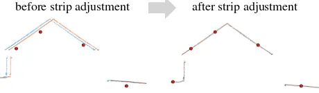
The main components of an ALS system are a laser scanner, a Global Navigation Satellite System (GNSS), and an Inertial Nav-igation System (INS). The GNSS and INS measurements serve to estimate the aircraft’s trajectory, i.e. its position (three coordi-nates) and its orientation (three angles). Using the trajectory, the mounting calibration parameters (which describe the positional and rotational offset between the scanner and the GNSS/INS sys-tem), and the measurements of the scanner (range and angle(s)), the 3d coordinates of the surface points can be determined. Sys-tematic errors in any of these data inputs lead to a sysSys-tematic, usually nonlinear deformation of the strip wise collected point clouds. These errors can be recognized in two forms: as discrep-ancies between overlapping strips and as discrepdiscrep-ancies between strips and ground-truth data, e.g. ground control points. Using strip adjustment, the quality of the ALS point clouds can be im-proved by simultaneously minimizing these discrepancies (Fig-ure 1).
before strip adjustment after strip adjustment
Figure 1: The discrepancies between overlapping strips (blue/orange) and between strips and ground control points (red) are minimized simultaneously by strip adjustment.
Parts of the strip adjustment method presented in this article are based on the Iterative Closest Point (ICP) algorithm (Besl and McKay (1992), Chen and Medioni (1992)). This algorithm is used to improve the alignment of two (or more) point clouds by minimizing iteratively the discrepancies within the overlap area
∗Corresponding author
of these point clouds. Nowadays the term ICP does not necessar-ily refer to the algorithm presented in the original publications, but rather to a group of surface matching algorithms which have in common the following aspects:
I : correspondences are establishediteratively
C: as correspondence the closest point, or more generally, the correspondingpoint, is used
P: correspondences are established on apoint basis.
The key features of the presented strip adjustment method are:
Calibration of the ALS multisensor system The scanner’s in-terior calibration and the mounting calibration are re-estimated in the strip adjustment. For this, additional calibration parameters are introduced into the general formulation of the direct georefer-encing equation. This approach is rigorous, as the original scan-ner measurements and the trajectory of the aircraft are used as inputs.
Correction of the aircraft’s trajectory The trajectory of the aircraft is considered to be estimated in advance from the GNSS and INS measurements (e.g. using some sort of Kalman filter (Hebel and Stilla, 2012)). As these measurements are affected by external influences (e.g. number of satellites), their accuracy is not constant, but dynamically changing. In order to reduce any possible systematic errors, trajectory correction parameters are estimated for each ALS strip individually.
Point based correspondences In order to exploit the full res-olution of the data, correspondences are established on the basis of the original ALS points. A single correspondence is defined by two points and their normal vectors. In the Least Squares Ad-justment, the point-to-plane distances of all correspondences are minimized simultaneously.
iterative procedure is repeated until convergence is reached, i.e. there are no significant changes in the estimated parameters.
Moreover, the presented method is suitable for large amounts of data (up to a few hundreds of strips), is fully automatic, and has no restriction on the object space in terms of shape. If available, ground-truth data can be considered.
The rest of the paper is organized as follows. After a review of re-lated literature in section 2., the general formulation of the direct georeferencing process and its refinement with additional param-eters is presented in section 3. On this basis, the strip adjustment method is presented in section 4. This includes a detailed de-scription of the correspondences and the functional and stochas-tic model of the adjustment. In section 5., the strip adjustment method is demonstrated on the basis of an ALS block consisting of 103 strips. The conclusions are presented in the last section.
2. RELATED WORK
Basically, two types of strip adjustment methods exist: (a) rubber-sheeting coregistration solutions, which use the measured terrain points only as input (Ressl et al., n.d.) and (b) rigorous solu-tions that start from the original scanner and trajectory measure-ments. Rigorous solutions, as the one presented in this article, differ mainly in terms of the estimated parameters and the used correspondences. Many methods concentrate on the estimation of the misalignment between the scanner and the INS (Hebel and Stilla, 2012; Toth, 2002). The most extensive parameter models are presented in Kager (2004) and Friess (n.d.). Correspondences are either generated on the basis of the original point cloud or a derivate of it (e.g interpolated grids or triangulations). Most ap-proaches use planes as corresponding geometric elements. They can be of fixed size or variable size found by segmentation (e.g. rooftops). Kersting et al. (2012) use higher order primitives as correspondences. An overview of strip adjustment methods is presented in Toth (2009) and Habib and Rens (2007).
3. DIRECT GEOREFERENCING
3.1 General formulation
The direct georeferencing of ALS strips requires three data in-puts: the scanner measurements, the trajectory of the aircraft, and the mounting calibration parameters (Skaloud and Lichti, 2006; Hebel and Stilla, 2012). Combining all these measurements, the point coordinates at timetare given by
xe(t) =ge(t) +Ren(t)R n i(t)
ai+Risx s
(t) (1)
In this representation the superscript of a vector denotes the coor-dinate system in which it is defined, whereas the notationRtarget source is used to denote a transformation from asourcecoordinate sys-tem to atargetcoordinate system. Consequently, four coordinate systems appear in equation (1):
s-system scanner coordinate system
i-system INS coordinate system, sometimes also denoted as body coordinate system
n-system navigation coordinate system, equal to a local-level coordinate system
e-system Earth-Centered, Earth-Fixed (ECEF) coordinate system
Definitions of these coordinate systems can be found in B¨aumker and Heimes (n.d.). Furthermore, equation (1) includes:
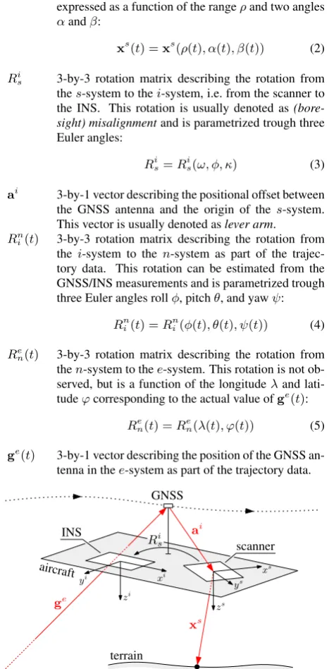
xs(t) 3-by-1 vector with the coordinates of the laser point in thes-system. Generally, these coordinates can be expressed as a function of the rangeρand two angles αandβ:
xs(t) =xs(ρ(t), α(t), β(t)) (2)
Ri
s 3-by-3 rotation matrix describing the rotation from thes-system to thei-system, i.e. from the scanner to the INS. This rotation is usually denoted as (bore-sight) misalignmentand is parametrized trough three Euler angles:
Ris=R i
s(ω, φ, κ) (3)
ai 3-by-1 vector describing the positional offset between the GNSS antenna and the origin of the s-system. This vector is usually denoted aslever arm.
Rn
i(t) 3-by-3 rotation matrix describing the rotation from the i-system to the n-system as part of the trajec-tory data. This rotation can be estimated from the GNSS/INS measurements and is parametrized trough three Euler angles rollφ, pitchθ, and yawψ:
Rni(t) =R n
i(φ(t), θ(t), ψ(t)) (4)
Re
n(t) 3-by-3 rotation matrix describing the rotation from then-system to thee-system. This rotation is not ob-served, but is a function of the longitudeλand lati-tudeϕcorresponding to the actual value ofge(t):
Rne(t) =Ren(λ(t), ϕ(t)) (5)
ge(t) 3-by-1 vector describing the position of the GNSS an-tenna in thee-system as part of the trajectory data.
GNSS
INS
scanner
aircraft
terrain ge
ai
xs zi
xi yi
zs ys
xs Ris
Figure 2: Direct georeferencing of ALS point clouds.
It should be noted, that the strip adjustment method presented herein is fully performed in thee-system. Only afterwards, the points obtained by equation (1) are projected from thee-system to an arbitrary mapping coordinate system (m-system), e.g. UTM. This has the main advantage that the surface distortions applied in them-system have not to be considered in the strip adjustment.
Side note If the trajectory is provided by an external company, in most of the cases it already relates to thes-system (in contrast to the definition given above). In this case
• the angles rollφ, pitchθ, and yawψdirectly describe the rotation from thes-system to then-system:
Rns(t) =R n i(t)R
i s=R
n
s(φ(t), θ(t), ψ(t)) (6)
• and the lever armaican be omitted in equation (1).
As a result, equation (1) simplifies to:
xe(t) =ge(t) +Ren(t)R n s(t)x
s
(t) (7)
3.2 Additional parameters
Any measurement in equation (1) can be affected by systematic errors, which in turn cause a systematic (nonlinear) deformation of the ALS strip (Glennie, 2007; Habib and Rens, 2007). To minimize these errors within the strip adjustment, additional cal-ibration and correction parameters have to be introduced into the direct georeferencing equation (1). These parameters can be di-vided into three groups:
Scanner calibration parameters The scanner calibration pa-rameters compensate for the systematic errors of the ALS scan-ner’s measurementsxs. The estimation of these parameters within the adjustment is usually denoted ason-the-job calibration. A comprehensive analysis of scanner related errors and their causes can be found in Katzenbeisser (n.d.). The specific choice of pa-rameters primarily depends on the construction type of the ALS scanner, especially on its beam deflection mechanism. For ex-ample, the parameters required to appropriately model the errors of scanners that deflect the laser beam only in one direction (lin-ear scanners), differ from those that deflect the laser beam in a circular pattern (nutating scanners). Hence, no general recom-mendation can be given. Instead, we propose a calibration model which is universally applicable, although it may not be the opti-mal choice in any case. Therefore we formulatexs, according to equation (2), as a function of the polar coordinatesρ,α, andβ:
xs(t) =
ρ(t) cosα(t) sinβ(t)
ρ(t) sinα(t)
ρ(t) cosα(t) cosβ(t)
s
(8)
For each polar coordinate two calibration parameters are intro-duced, an offset and a scale. This yields to three offset parameters (∆ρ,∆α,∆β) and three scale parameters (ερ,εα,εβ) which are defined by
ρ(t) = ∆ρ+ρ0(t) ·(1 +ερ) (9) α(t) = ∆α+α0(t)·(1 +εα) (10) β(t) = ∆β+β0(t)·(1 +εβ) (11)
where the original scanners’s measurements are denoted byρ0, α0, andβ0.
EXAMPLELinear scanners deflect the laser beam only in one di-rection (usually across the flight track). Thus,αcan be inter-preted as the beam deflection angle, whereasβis equal to zero. The parameters associated withβ, i.e.∆βandεβ, can be omitted in this case. The remaining parameters compensate for a range finder offset error (∆ρ), a range finder scale error (ερ), a zero-point error of the angular encoder (∆α), and a scale error of the angular encoder (εα). However, these parameters may also com-pensate for other correlated (and possibly unknown) effects. For example, the parameterεαnot only serves to correct an angular scale error, but also minimizes the influence of the atmospheric refraction. Similarly, the parameterερ, which primarily corrects a range finder scale error, may also compensate range errors caused by the atmospheric propagation delay.
Trajectory correction parameters The trajectory of the air-craft, i.e. its orientationRinand its positiong
e
, is estimated by
the integration of GNSS and INS measurements in a Kalman fil-ter. Skaloud et al. (2010) highlight the fact that all these mea-surements are strongly affected by external influences and hence their accuracy can not be assumed to be constant in time. As these systematic trajectory errors even varywithina single ALS strip, time dependent correction parameters should be estimated for each strip. However, the determinability of such parameters strongly depends on the terrain geometry and can not be guar-anteed in any case (e.g. over flat terrain). We therefore limit the estimation on the constant part of the trajectory errors for each strip. For this an individual set of six trajectory correction pa-rameters (three angle corrections and three position corrections) is assigned to each strip. The angle corrections (∆φi,∆θi,∆ψi) for stripiare defined by
φ(t) =φ0(t) + ∆φi (12) θ(t) =θ0(t) + ∆θi (13) ψ(t) =ψ0(t) + ∆ψi (14)
whereφ0,θ0, andψ0denote the original values of the roll, pitch, and yaw angles. Accordingly, the position corrections (∆gxi, ∆gyi,∆gzi) for stripiare defined by
ge(t) =ge0(t) + ∆g e
=
gx0(t) + ∆gxi gy0(t) + ∆gyi gz0(t) + ∆gzi
e
(15)
wheregx0,gy0, andgz0denote the original position values.
Mounting calibration parameters In most of the cases the mounting calibration parameters, that is the misalignmentRi
sand the lever-armai, are already known in advance, e.g. from a pre-viously performed calibration or from construction plans of the system. However, these values can be inaccurate or outdated. Thus, it is recommended to re-estimate the mounting calibration by strip adjustment. Especially an incorrect misalignment, which is difficult to measure by terrestrial measurements, can cause very large point displacements, because the effect of angular errors is directly proportional to the object distanceρ. For this rea-son many strip adjustment methods concentrate on the estimation ofRi
s, neglecting other parameters (e.g. Toth (2002), Hebel and Stilla (2012)). The mounting calibration parameters are already included in equation (1), where the misalignmentRisis defined by the anglesω,φ,κ, and the lever-arm is defined by the compo-nents ofai, namelyax,ay, andaz.
Summarizing, the following parameters can be estimated within the proposed strip adjustment:
• Scanner calibration parameters – range and angle offsets∆ρ,∆α,∆β
– range and angle scalesερ, εα, εβ
• Trajectory correction parameters(for each stripi) – angle corrections∆φi,∆θi,∆ψi
– position corrections∆gxi,∆gyi,∆gzi
• Mounting calibration parameters – misalignment anglesω, φ, κ
– lever-arm componentsax, ay, az
4. STRIP ADJUSTMENT
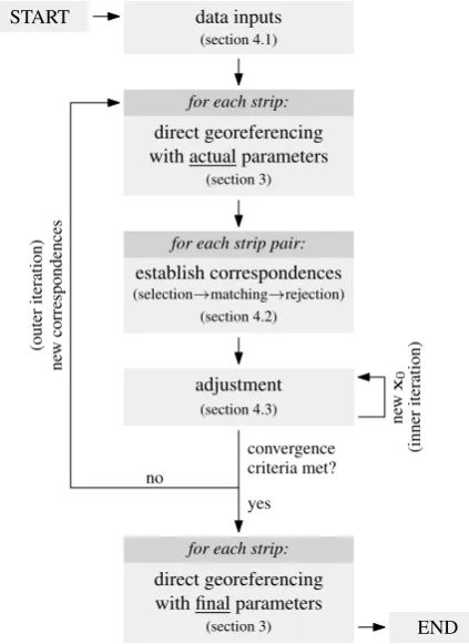
The main steps of the strip adjustment method are shown in Fig-ure 3. As it can be seen, two iteration loops exist: within the outer iteration loop the correspondences are re-established (as in the ICP algorithm) after each run, whereas the inner iteration loop is needed to solve the non-linear equation system within the ad-justment. In the following sections, the data inputs, the corre-spondences, and the adjustment are described in detail.
direct georeferencing with actual parameters
establish correspondences for each strip:
(selection→matching→rejection) (section 4.2) for each strip pair:
adjustment (section 3)
(section 4.3)
START data inputs
(section 4.1)
direct georeferencing with final parameters
for each strip:
(section 3) END convergence
criteria met?
yes no
ne
w
x0
(inner
iteration)
ne
w
correspondences
(outer
iteration)
Figure 3: Flowchart of strip adjustment method.
4.1 Data inputs
The following data inputs are used in the strip adjustment:
• Scanner measurements:xs(t)
• Trajectory of the aircraft:ge(t)andRn i(t)
• Mounting calibration parameters:Risandai
These values are introduced as approximations in the Least Squares Adjustment. If noa prioriinformation about the mounting calibration exists, then the misalignmentRisshould be chosen so that itapproximatelyrotates thes-system into thei-system, whereas the lever-armaican be approximated by the null vector.
• Ground-truth data(optional, see section 4.4)
4.2 Correspondences
As demonstrated in Glira et al. (2015), the strip adjustment re-sults are strongly affected by the used correspondences. We pro-pose to establish the correspondences on the basis of the original ALS points; the main reasons for this are: the highest possible resolution level of the data is exploited, no time-consuming pre-processing of the data is required (in contrast to correspondences which are found by segmentation and/or interpolation), and no restrictions are imposed on the object space (e.g. the presence of rooftops or horizontal fields). A single correspondence is de-fined by two points from overlapping strips and their normal vec-tors (estimated from the neighbouring points). As a point and its
normal vector define a tangent plane, consequently, a correspon-dence represents two homologous tangent planes in object space. In the Least Squares Adjustment the so-called point-to-plane dis-tance, which is defined as the perpendicular distance from one point to the tangent plane of the other point, is minimized.
The correspondences are established for each pair of overlapping strips in three distinct steps: theSelection, Matching, and Re-jectionstep. A comprehensive description of these steps can be found in Glira et al. (2015). Thus, only a brief summary is pro-vided here.
Selection In this step, a subset of points is selected within the overlap area in one strip. For this task four selection strategies are considered. The main difference between these strategies is the information used as input for the point selection; see Table 4.2. The four selection strategies, sorted by increasing computational complexity, are:
• Random Sampling (RS) This is the fastest strategy, be-cause points are simply selected randomly, without consid-ering the coordinates or the normal vectors of the points. For ALS point clouds, in which the point density is nearly con-stant, this option can be considered as an approximation of uniform sampling.
• Uniform Sampling (US)The aim of this strategy is to select points in object space as uniformly as possible. This leads to a homogeneous distribution of the selected points, where regions of equal area are equally weighted within the adjust-ment. On the contrary, if a normal direction is predominat-ing (e.g. flat terrain), many redundant points with approxi-mately parallel normal vectors, which do not contribute sig-nificantly to the parameter estimation, are selected. This op-tion was implemented by dividing the overlap area into a voxel structure and selecting the closest point to each voxel center. Consequently, the edge length of a single voxel can be interpreted as the mean sampling distance along each co-ordinate direction.
• Normal Space Sampling (NSS)The aim of this strategy is to select points such that the distribution of their normals in angular space is as uniform as possible (Rusinkiewicz and Levoy, 2001). For this the angular space (slope vs. aspect) is divided into classes (e.g. 2.5°x10°), and points are ran-domly sampled within these classes. This strategy does not consider the position of the points.
• Maximum Leverage Sampling (MLS) This strategy se-lects those points, which are best suited for the estimation of the parameters. For this, the effect of each point on the parameter estimation, i.e. its leverage, is considered. The points with the maximum leverage (= the lowest redundancy) are selected. This strategy considers the coordinates and the normal vectors of the points. Details on the algorithm can be found in Glira et al. (2015).
RS US NSS MLS
coordinates of points no yes no yes normal vectors of points no no yes yes
Table 1: Information used by the selection strategies.
(e.g. urban area, hilly or mountainous terrain; see example in sec-tion 5.). However,NSSconsiders the normal vectors and thus a sufficient number of points is selected within the ditch. MLS additionally evaluates the coordinates of the points in order to es-timate the leverage of each point on the parameter estimation. As a result, points are primarily selected in the ditch and towards the edges of the overlap area.
ditch almost flat terrain
Random Sampling (RS)
Uniform Sampling (US)
Normal Space Sampling (NSS)
Max Leverage Sampling (MLS)
Figure 4: Comparison of correspondence selection strategies (from Glira et al. (2015)). Each strategy was applied to select approximately 300 points. A shaded Digital Elevation Model (DEM) of the ALS scene is visualized in the background.
Matching This step establishes the correspondences. For this, each selected point from the previous step is paired to the near-est neighbour (closnear-est point) of the overlapping strip. As in the adjustment the point-to-plane distance is minimized for each cor-respondence, two associated points don’t have to be identical in object space, but they only have to belong to the same (tangent) plane (e.g. flat terrain surface). Due to the good initial orientation and the high point density in ALS, this requirement is mostly ful-filled. The nearest neighbour search can be realized efficiently using k-d trees.
Rejection The aim of this step is thea prioriidentification and subsequent rejection of unreliable or false correspondences. Each correspondence is tested for three criteria:
• Rejection based on the plane roughness of corresponding pointsFor the minimization of the point-to-plane distance, the reliability of both normal vectors must be ensured. Of course, this condition is not met if the scanned object can not be appropriately modelled by a plane, e.g. in the case of vegetation. This is directly reflected by thea posteriori reference varianceσˆ20 of the tangent plane adjustment. We denote the standard deviationσˆ0as the plane roughness and reject all correspondences where at least one of the twoˆσ0 values exceeds an upper limitσmax. We usually setσmax= 10 cm.
• Rejection based on the angle between the normal vectors of corresponding pointsTo ensure that two corresponding points belong to the same plane, the angleαbetween the normal vectors of these points should not exceed an upper limitαmax. We usually setαmax= 5°.
• Rejection based on the point-to-plane distance between corresponding pointsApart from a few false correspon-dences, thea prioripoint-to-plane distancesd1,d2, . . . ,dn are assumed to be normally distributed for each individual pair of overlapping strips. A robust estimator for the stan-dard deviation of this contaminated set of correspondences is given by
σmad= 1.4826·mad (16)
where mad is the median of the absolute differences (with
respect to the median) (Hampel, 1974). In this work, all correspondences with a point-to-plane distance outside the range ofd˜±3σmadare rejected, whered˜denotes the median of the point-to-plane distances of all correspondences that passed the first two criteria.
It is not guaranteed that all false correspondences are rejected by this three criteria. Thus, a robust adjustment method is used for the detection and removal of the remaining ones.
4.3 Adjustment
A robust Least Squares Adjustment is performed in order to es-timate the parameters described in section 3.2. The objective of the adjustment is to minimize the weighted sum of squared point-to-plane distances
Ω=
n
X
i=1
(wid2i)→minimum (17)
wherewiis the weight, anddiis the point-to-plane distance of thei-th correspondence. In the following, the definitions ofwi (stochastic model) anddi(functional model) are given.
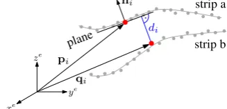
Definition of point-to-plane distance The signed point-to-plane distance di (Figure 5) is defined as the perpendicular distance from a point to a plane. It is conveniently expressed by the Hes-sian normal form
di= (pi−qi)Tni (18)
wherepiandqi are the corresponding points of thei-th corre-spondence, andniis the normal vector associated to the pointpi (with||ni||= 1). In this eq. the pointspiandqiare determined by the direct georeferencing equation (1), i.e. in consideration of the scanner measurements, the trajectory, the mounting cal-ibration parameters, and the additional parameters described in section 3.2.
plane
di
ni
pi
qi
strip a
strip b ze
xe
ye
Figure 5: The point-to-plane distancedifor thei-th correspon-dence is defined as the perpendicular distance from pointqito the tangent plane defined bypiandni. The pointqiis the nearest neighbour of the pointpi.
strip pairk, then its weight is determined by
wi= 1
σ2 k
(19)
whereσk is theσmad value (16) of all (non-rejected) point-to-plane distances belonging to the strip pairk.
Adjustment solution The functional model of the adjustment evolves from the condition, that for each pair of corresponding points(pi,qi), the pointqi should be in the tangent plane of pointpi. In other words, the point-to-plane distancesdi(cf. eq. (18)) should be equal to zero for allncorrespondences. This can be formulated for each individual correspondence by writing
di= 0 +vi for i= 1, . . . , n (20)
wherevidenotes the residual distance after adjustment. From thesenequations, the u-dimensional parameter vectorxis es-timated in consideration of the objective function stated in (17). For this, we rewrite the equation system (20) in vector notation, whereby the point-to-plane distancesdiare expressed as a func-tion of the estimated parametersxˆ
f(ˆx) =v (21)
In order to resolve this equation system for the parametersˆx, the nonlinear functionsf(ˆx)must be linearized by
f(ˆx) =f(x0) + ∂f(x)
∂x
x=x0
·∆ˆx=f(x0) +A∆ˆx (22)
wherex0 denotes the vector of approximate parameter values, andAdenotes then-by-udesign matrix which includes the par-tial derivatives of the equations with respect to the parameters at the pointx0. The parameter estimatesˆxand the residualsvcan then be determined by the equations
ˆ
x=x0+ ∆ˆx (23)
v=A∆ˆx (24)
with
∆ˆx= (ATP A)−1
ATP(−f(x0)) (25) and
P=diag(w1, . . . , wn) (26)
The iterative process of relinearization terminates when∆ˆx be-comes insignificantly different to zero (inner iteration, cf. Fig-ure 3). We use the termination criterion described in (Kraus, 1997, p. 76).
In order to identify wrong correspondences (outliers), al1-norm minimization is imitated within the adjustment by iteratively weighting the observations (Kraus, 1997, p. 218). After the re-moval of the detected outliers, a final regular Least Squares Ad-justment is performed with the remaining correspondences (in-liers). The amount of outliers strongly depends on the input data, but typically does not exceed 5%.
4.4 Datum definition and ground-truth data
The datum of the ALS block can be defined in two ways: (a) by fixing the trajectory of one or more strips (i.e. by omitting the trajectory correction parameters of these strips) or (b) by con-sidering ground-truth data (if available). Ground-truth data can be provided in many forms, e.g. as single (widely isolated) points from total station or GNSS measurements, as georeferenced point clouds from Terrestrial Laser Scanning (TLS), or as a DEM to which the ALS block should fit. Thus, a flexible concept, that can
handle all these possibilities, is needed. We propose to treat the various forms of ground-truth data simply as further point clouds, whose orientations are fixed in object space. Additional cor-respondences between ground-truth data and overlapping ALS strips are introduced by equation (18), whereby the ground-truth data is represented by the pointsqi. Usingqi (instead ofpi) for the ground-truth data has the major advantage, that the nor-malsniare estimated from the ALS points, and thus also isolated points (with unknown normal vector) can be used as ground-truth data.
5. EXPERIMENTAL RESULTS
The presented strip adjustment method was applied to an ALS block located in the Austrian Alps (Tyrol, Kaunertal, Gepatsch-ferner). The block consists of 95 longitudinal strips and 8 cross strips (Figure 6 (a)); the cross strips were flown in both direc-tions. The ALS system was carried by a helicopter that flew over the terrain in a constant height above ground of approx. 600 m. Further information about the flight campaign is summarized in Table 5.. A quality control of the delivered data revealed large systematic discrepancies (of up to several dm) in the overlap area of neighbouring strips. For this reason, an improvement of the georeferencing of the data by means of strip adjustment, was ab-solutely necessary.
scanner model Riegl LMS-Q680i
area of ALS block approx. 119 km2
no. of strips 103
no. of ground-truth data areas 4
size of input data 58.8 GB
overall no. of points 1 455 111 768 mean point density (single strip) 2.5 points/m2 mean point density (block) 12.2 points/m2 frequency of trajectory data 256 Hz
terrain elevation 2100 to 3450 m
Table 2: Key parameters of the ALS data used.
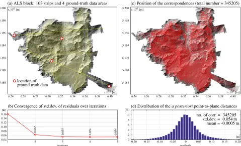
Next to the georeferenced strips, also the original scanner mea-surements and the trajectory data were provided. However, no a priori information about the mounting calibration was avail-able. Thus, approximate values for these parameters were de-termined as described in section 4.1. In total, 627 parameters were estimated in the adjustment; this includes 3 scanner calibra-tion parameters (range offset∆ρ, range scaleερ, scan angle scale εα), 6 mounting calibration parameters, and 6 trajectory correc-tion parameters for each of the 103 strips. As it can be seen in Figure 6 (b), five correspondence iterations (cf. Figure 3) were performed within the strip adjustment, although three iterations would have been sufficient. The reason for this is that we used, instead of a convergence criteria based e.g. on the change of the parameter estimatesxˆ after each iteration, a fixed number of 5 correspondence iterations.
location of ground truth data 5.188
x 106 [m]
6.24
x 105[m] 6.26 6.28 6.30 6.32 6.34 6.36 6.38 6.40 5.190
5.192 5.194 5.196 5.198 5.200
5.188
6.24 6.26 6.28 6.30 6.32 6.34 6.36 6.38 6.40 5.190
5.192 5.194 5.196 5.198 5.200
2 4 6 8 10
0 x 106
[m]
x 105[m]
[%]
-0.20 -0.15 -0.10 -0.05 0 0.05 0.10 0.15 0.20 [m]
1 2 3 4 5 0
0.04 0.06 0.08 0.10 0.12 0.14 0.16 [m]
iterations residuals
0.062
0.055 0.054 0.054
(a) ALS block: 103 strips and 4 ground-truth data areas (c) Position of the correspondences (total number = 345205)
(d) Distribution of thea posterioripoint-to-plane distances (b) Convergence of std.dev. of residuals over iterations
std.dev. = 0.054 m mean = -0.0005 m no. of corr. = 345205
Figure 6: Strip adjustment results for an ALS block covering an area of approx. 119 km2in the Austrian Alps (Kaunertal).
normally distributed, which indicates that systematic errors were widely eliminated by strip adjustment and confirms the appro-priateness of the applied transformation model. In Figure 7 the mean and the standard deviation of these residuals are visualized individually for each strip pair. The strip pairs are thereby or-dered by decreasing number of correspondences. As expected, the magnitude of the mean values is increasing by decreasing no. of correspondences (which is equivalent to a decreasing weight of the strip pairs), whereas the standard deviation remains, mainly due to the homogeneity of the terrain and of the surveying condi-tions, nearly constant.
The datum of the ALS block was defined by 4 ground-truth data areas (Figure 6 (a)). Altogether, these areas consist of 205 points, which were chosen predominantly on roofs and streets and were determined by a combination of static GNSS and total station measurements. These points were matched with 24 overlapping strips, giving in total 632 datum-defining (“ground-truth data to strip”) correspondences.
no. of estimated parameters 627
no. of iterations 5
no. of overlapping strip pairs 748 no. of correspondences (“strip to strip”) 345205
→mean of residuals -0.0005 m
→std.dev. of residuals 0.054 m
no. of correspondences (“gtd to strip”) 632
→mean of residuals -0.0002 m
→std.dev. of residuals 0.053 m
Table 3: Strip adjustment results (gtd = ground-truth data).
6. SUMMARY AND OUTLOOK
We presented a new strip adjustment method which:
0 100 200 300 400 500 600 700
0 4000 3000 2000 1000
(a) Number of correspondences for each strip pair
0 100 200 300 400 500 600 700
-0.04 0.04 0.02 0 -0.02
(b) Mean ofa posterioripoint-to-plane distances
0 100 200 300 400 500 600 700
0 0.20 0.15 0.10 0.05
(c) Std. dev. of thea posterioripoint-to-plane distances
[m]
strip pair index
strip pair index
[m]
total number of strip pairs = 748
strip pair index
Figure 7: Strip adjustment results for all 748 overlapping strips pairs. The strip pairs are ordered according to the no. of corre-spondences.
• is formulated in a mathematically rigorous way, i.e. the orig-inal scanner measurements and the trajectory are used as data inputs
• estimates the ALS scanner calibration parameters
• estimates the mounting calibration of the ALS scanner
• corrects the aircraft’s trajectory individually for each strip
• uses correspondences on the basis of the original ALS points
• establishes the correspondences not only once, but itera-tively until convergence is reached
• minimizes simultaneously the point-to-plane distances of all correspondences
strips)
• is robust against false correspondences (outliers)
• considers ground-truth data in most forms, e.g. single ground control points or DEMs
• poses no restrictions on the object space in terms of shape (e.g. the presence of rooftops or horizontal fields)
• is fully automatic.
The suitability of the method for large amounts of data was demon-strated on the basis of a larger ALS block, in which systematic discrepancies were widely eliminated. Currently, we are working on the following extensions of the presented method:
1. Time-dependent trajectory correction parameters In rare cases, the trajectory measurements can be of very poor quality, i.e. the accuracy of the trajectory is highly vari-able, even within a single strip. In such cases, the trajectory correction parameters described in section 3.2 might not be sufficient, as they only compensate the errorson averagefor each strip. Thus, we plan to extend the parameter model by time-dependent trajectory correction parameters.
2. Synchronization error between scanner and trajectory As the scanner and trajectory measurements stem from dif-ferent sensors, it may occur that they are not correctly syn-chronized (Katzenbeisser, n.d.). Such a synchronization er-ror can cause discrepancies between overlapping strips in the order of a few dm. This error can be estimated and cor-rected by means of strip adjustment.
3. RANSAC based rejection of false correspondences The rejection of unreliable or false correspondences is scribed in section 4.2. In order to further improve the de-tection of these outliers, we plan to additionally apply a new rejection method which is based on the RANSAC algorithm.
The strip adjustment method presented herein will be integrated into the software package OPALS (Pfeifer et al., 2014).
ACKNOWLEDGEMENTS
The authors would like to thank Mr. Helmuth Kager for his valu-able contributions to this project. This research was carried out within the project PROSA (high-resolution measurements of mor-phodynamics in rapidly changing PROglacial Systems of the Alps) which is a joined project of the German research community (DFG) (BE 1118/27-1) and the Austrian Science Fund (FWF) (I 1647).
References
B¨aumker, M. and Heimes, F., n.d. New calibration and com-puting method for direct georeferencing of image and scanner data using the position and angular data of an hybrid inertial navigation system. In: OEEPE Workshop, ”Integrated Sensor Orientation”, Hannover, Germany.
Besl, P. J. and McKay, N. D., 1992. Method for registration of 3-d shapes. In: Robotics-DL tentative, International Society for Optics and Photonics, pp. 586–606.
Chen, Y. and Medioni, G., 1992. Object modelling by registration of multiple range images. Image and Vision Computing 10(3), pp. 145 – 155. Range Image Understanding.
Friess, P., n.d. Toward a rigorous methodology for airborne laser mapping. In: Proceedings EuroCOW, Castelldefels, Spain.
Glennie, C., 2007. Rigorous 3d error analysis of kinematic scan-ning lidar systems. Journal of Applied Geodesy 1(3), pp. 147– 157.
Glira, P., Pfeifer, N., Ressl, C. and Briese, C., 2015. A correspon-dence framework for als strip adjustments based on variants of the ICP algorithm. Journal for Photogrammetry, Remote Sens-ing and Geoinformation Science (accepted).
Habib, A. and Rens, J., 2007. Quality assurance and quality con-trol of lidar systems and derived data. In: Advanced Lidar Workshop, University of Northern Iowa, United States.
Hampel, F. R., 1974. The influence curve and its role in robust estimation. Journal of the American Statistical Association 69(346), pp. 383–393.
Hebel, M. and Stilla, U., 2012. Simultaneous calibration of ALS systems and alignment of multiview LiDAR scans of urban ar-eas. Geoscience and Remote Sensing, IEEE Transactions on 50(6), pp. 2364–2379.
Kager, H., 2004. Discrepancies between overlapping laser scan-ner strips–simultaneous fitting of aerial laser scanscan-ner strips. In-ternational Archives of Photogrammetry, Remote Sensing and Spatial Information Sciences 35(B1), pp. 555–560.
Katzenbeisser, R., n.d. About the calibration of lidar sensors. In: ISPRS Workshop ”3-D Reconstruction form Airborne Laser-Scanner and InSAR data”; 8-10 Oct. 2003, Dresden, Germany.
Kersting, A. P., Habib, A. F., Bang, K.-I. and Skaloud, J., 2012. Automated approach for rigorous light detection and ranging system calibration without preprocessing and strict terrain cov-erage requirements. Optical Engineering 51(7), pp. 076201–1.
Kraus, K., 1997. Photogrammetry, Vol.2, Advanced Methods and Applications. Duemmler / Bonn.
Pfeifer, N., Mandlburger, G., Otepka, J. and Karel, W., 2014. OPALS – A framework for airborne laser scanning data anal-ysis. Computers, Environment and Urban Systems 45(0), pp. 125 – 136.
Ressl, C., Pfeifer, N. and Mandlburger, G., n.d. Applying 3D affine transformation and least squares matching for airborne laser scanning strips adjustment without GNSS/IMU trajectory data. In: Proceedings of ISPRS Workshop Laser Scanning 2011, Calgary, Canada.
Rusinkiewicz, S. and Levoy, M., 2001. Efficient variants of the ICP algorithm. In: 3-D Digital Imaging and Modeling, 2001. Proceedings. Third International Conference on, Quebec City, Canada, pp. 145–152.
Skaloud, J. and Lichti, D., 2006. Rigorous approach to bore-sight self-calibration in airborne laser scanning. ISPRS journal of photogrammetry and remote sensing 61(1), pp. 47–59.
Skaloud, J., Schaer, P., Stebler, Y. and Tom´e, P., 2010. Real-time registration of airborne laser data with sub-decimeter accuracy. ISPRS Journal of Photogrammetry and Remote Sensing 65(2), pp. 208–217.
Toth, C. K., 2002. Calibrating airborne lidar systems. In: IS-PRS Commission II, Symposium 2002, Xian, China, ISIS-PRS Archives, Volume XXXIV Part 2, pp. 475–480.