www.elsevier.nl / locate / econbase
Incentive effects of social security on labor force
participation: evidence in Germany and across Europe
* ¨
Axel Borsch-Supan
Department of Economics, University of Mannheim, 68131 Mannheim, Germany
Abstract
All across Europe, old age labor force participation has declined dramatically during the last decades. This secular trend coincides with population aging. The European social security systems therefore face a double threat: Retirees receive pensions for a longer time while there are less workers per retiree to shoulder the financial burden of the pension systems. This paper shows that a significant part of this problem is homemade: most European pension systems provide strong incentives to retire early. The correlation between the force of these incentives with old age labor force participation is strongly negative. The paper provides qualitative and econometric evidence for the strength of the incentive effects on old age labor supply across Europe and for the German public pension program. 2000 Elsevier Science S.A. All rights reserved.
Keywords: Labor force participation; Social security; Incentive; Pensions
1. Introduction
Pay-as-you-go (PAYG) systems dominate the old age social security programs in Europe. French, German and Italian workers rely almost exclusively on pensions financed by a PAYG system, while the Netherlands and Great Britain are exceptions in funding a substantial fraction of their future pension benefits. In the Netherlands, defined benefit plans dominate. As has been stressed quite frequently (OECD, 1988), the population aging process puts all pension systems under severe
*Fax: 11-149-621-292-5426.
¨
E-mail address: [email protected] (A. Borsch-Supan).
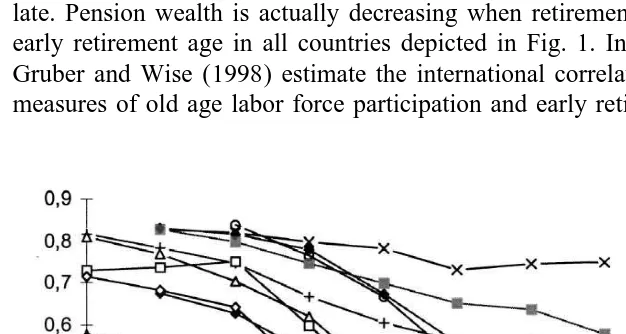
age labor force is strongly correlated with the incentives created by generous early retirement provisions. Unlike defined contribution plans in funded pension systems, pay-as-you-go systems are intrinsically difficult to design in a fashion that is actuarially fair. Moreover, the early retirement provisions in most European pension systems increase this actuarial unfairness for those who retire normally or late. Pension wealth is actually decreasing when retirement is postponed past the early retirement age in all countries depicted in Fig. 1. In their summary article, Gruber and Wise (1998) estimate the international correlation between aggregate measures of old age labor force participation and early retirement incentives. Fig.
Fig. 1. Old age labor force participation in Europe, U.S. and Japan, 1960–1995. Note: labor force participation rates of men aged 60–64. Sources: Belgium: Pestieau and Stjins (1998); France: Blanchet
´ ¨
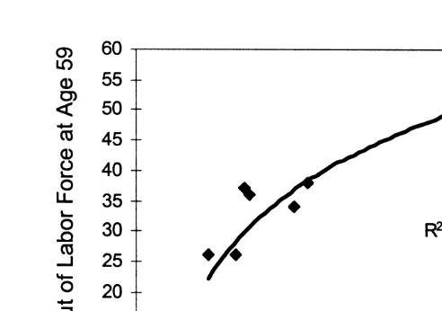
Fig. 2. Old age labor force participation disincentives and early retirement. Note: the measure of old age LFP disincentives sums the losses (gains) in pension wealth relative to the average wage, when retirement is postponed by a year over all years between the applicable early retirement age in each country and age 69. A value of 10 corresponds to 10 years with a tax rate of 100%. See Gruber and Wise (1998) for similarly well-fitting alternate specifications.
2 shows our variant of their results, linking the proportion of men out of labor force at age 59 with a measure of the strength of labor force disincentives after age 59, defined as the accumulated loss of pension wealth when retirement is postponed past age 59.
Fig. 2 is the starting point of this paper. Because it is dangerous to give the aggregate correlation in Fig. 2 a causal interpretation, this paper uses micro-economic evidence in order to continue the above line of reasoning and to go one more step in establishing causality. It claims that older workers in Europe have responded in a very systematic and consistent way to the early retirement provisions although the provisions varied considerably in their designs over time and across European countries.
The paper uses two strands of evidence to show this claim. One the one hand, it uses international variation in pension provisions across Europe to link incentives and labor force exit decisions. Countries included are Belgium, France, Germany, Italy, Spain, Sweden and the Netherlands. This part of the analysis uses no formal econometrics. Rather, it points out ‘kinks’ in the pension wealth accrual function. This key statistic of the first part of the paper relates the present discounted value of retirement benefits to retirement age. The paper shows that the institutional factors embedded in this function strongly correlate with ‘spikes’ in the departure rate from employment.
pension system, early retirement can be considerably reduced by abolishing early retirement incentives. Estimates for Germany indicate that an actuarial fair retirement system will reduce retirement before age 60 by more than a third. Second, the results imply that welfare comparisons between pay-as-you-go and fully funded systems that do not model the retirement decision ignore important welfare reducing redistributions between early and normal (and late) retirees.
The strategy of this paper is to employ several different ways to identify incentive effects, using historical, international and econometric evidence, in the hope that the weight of the cumulative evidence is stronger than the sum of each single step. The reader will therefore be shuttled among different perspectives. Section 2 begins with a brief description of the German pension system and the early retirement incentives it creates. Section 3 provides informal evidence for the link between early retirement incentives and old age labor force participation in Germany, and Section 4 extends this analysis to a set of European countries. Section 5 supplies the econometric methodology that is employed in Section 6 for a formal analysis of early retirement incentives in Germany, 1984–1996. Section 7 concludes.
2. Incentives created by the German public pension system
The German public pension system is particularly well-suited for a mi-croeconometric study of incentive effects on labor force participation because it is almost universal and we do not need to account for a variety of firm pension plans that create their own incentive effects but are usually not well captured in survey
¨
incomes that are currently about 70% of pre-retirement net earnings for a worker with a 45-year earnings history and average life-time earnings. This is substantial-ly higher than the corresponding U.S. net replacement rate of about 53%. In addition, the system provides relatively generous survivor benefits that constitute a substantial proportion of the total pension liability. As a result, social security income represents about 80% of household income of households headed by a person aged 65 and over, the remainder about equally divided among firm pensions, asset income, and private transfers.
Until 1972, retirement was mandatory at age 65. In 1972, several early retirement options were introduced, ‘early’ defined as before age 65, the ‘normal’ retirement age. This gives us a first time-series handle to identify potential incentive effects. The German public pension system now provides old-age
pensions for workers aged 60 and older and disability benefits for workers below
age 60, that are converted to old-age pensions latest at age 65. In addition,
pre-retirement (i.e., retirement before age 60) is possible using other parts of the
public transfer system, mainly unemployment compensation. A main feature of the German old-age pensions is ‘flexible retirement’ from age 63 for workers with a long service history. In addition, retirement at age 60 is possible for women, unemployed, and workers who cannot be appropriately employed for health or labor market reasons. This complicated system generates cross-sectional variation 1 that gives us another handle to identify how incentive effects alter labor supply.
Roughly 80% of the budget of the German public pension system is financed by contributions, the rest by federal government revenue. Contributions are collected like a payroll tax, levied equally on employees and employers. The contribution rate in 1998 is very high: 21% of monthly gross income, paid in equal parts by employer and employee. The tax base for these contributions is capped at about 180% of average wages.
Benefits are computed on a life-time contribution basis. They are the product of four elements: (1) the employee’s relative wage position, averaged over the entire earnings history, (2) the number of years of service life, (3) several adjustment factors, and (4) the average pension level. The first three factors make up the ‘personal pension base’ which is calculated when entering retirement. Note that pensions are proportional to length of service life, a unique feature of the German pension system. The fourth factor determines the income distribution between workers and pensioners in general and is adjusted annually to net wages. Thus, productivity gains are transferred each year to all pensioners, not only to new entrants. Due to a generous exemption, social security benefits are tax free unless income from other sources is high.
Early retirement incentives are created by the (lack of) adjustment factors. The 1972 pension rules do not have an explicit adjustment of benefits when a worker
1
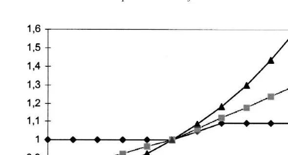
Fig. 3. Adjustment of retirement benefits to retirement age. Notes: ‘RR1972’ denotes adjustment factors under the 1972 legislation, and ‘RR1992’ to those that will eventually be phased in by the 1992 pension reform. ‘Fair’ refers to actuarially fair adjustment factors at a 3% discount rate.
retires earlier than at age 65, except for a bonus when retirement is postponed from ages 65 or 66 by 1 year, see Fig. 3. Nevertheless, because benefits are proportional to the years of service, a worker with fewer years of service will get lower benefits. With a constant income profile and 40 years of service, each year of earlier retirement decreased pension benefits by 2.5%. This is substantially less than the actuarial adjustment which increases from about 5.5% for postponing 2 retirement 1 year at age 60 to 8% for postponing retirement 1 year at age 65.
A key statistic to measure the early retirement incentives exerted by the actuarially unfair adjustment factors is the change in social security wealth. If social security wealth declines because the increase in the annual pension is not large enough to offset the shorter time of pension receipt, workers have a financial incentive to retire earlier. We define social security wealth as the expected present discounted value of benefits (YRET) minus applicable contributions that are levied on gross earnings (c?YLAB). Seen from the perspective of a worker who is S years old and plans to retire at age R, social security wealth (SSW) is
` R21
t2S t2S
SSW (R)S 5
O
YRET (R)t ?at?d 2O
c?YLABt?at?d ,t5R t5S
with:
2
SSW present discounted value of retirement benefits (5social security wealth)
S planning age
R retirement age,
YLABt gross labor income at age t
YRET (R) net pension income at age t for retirement at age Rt
ct contribution rate to pension system at age t
at probability to survive at least until age t given survival until age S
d discount factor51 /(11r).
The pension wealth accrual function, a function of the retirement age R, is the change in social security wealth when retirement is postponed from age R21 to age R:
ACCR (R)S 5[SSW (R)S 2SSW (RS 21)] / SSW (RS 21).
A negative accrual can be interpreted as a tax on further labor force participa-tion. We compute an implicit tax rate as the ratio of the (negative) social security
NET
wealth accrual to the net wages (YLAB ) that workers would earn if they would postpone retirement to age R:
NET TAXR (R)S 5 2[SSW (R)S 2SSW (RS 21)] / YLABR .
We use labor income after taxes in the denominator because workers presumably make their decision on postponing retirement by comparing potential losses in pension benefits (which are not taxed) to what they could earn net of taxes if they were staying in the labor force. The measure only includes the financial aspects of this decision. Alternatively, one might consider the consumption utility of net earnings and pension benefits and also account for the utility aspects of the labor–leisure tradeoff. We will do this further below when we will estimate the corresponding utility parameters in a sample of German workers and restrict the analysis in this part of the paper on the financial aspects only.
The implicit tax rate can be rewritten as the product of two terms. The first term represents the effect of postponing retirement through mortality, discounting, and the adjustment of benefits to retirement age, while the second term is the net
NET replacement rate YRET / YLABR R
TAXR (R)S 5[aR?d ?(c 21)21]?REPLR
If benefits are actuarially fair in a financial sense,c 5111 /aR?d, and the resulting tax rate is zero.
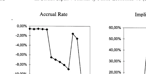
Fig. 4. Loss in social security wealth when postponing retirement, 1972 rules. Note: see text for definition of accrual rate ACCR (t) and implicit tax rate TAXR (t) for SS S 555 and t555 . . . 69.
generated by the bonus for postponing retirement at ages 65 and 66, interrupting the steady increase in negative pension wealth accrual.
The lack of actuarial fairness of the German public pension system creates a negative accrual of pension wealth during the early retirement window at a rate reaching29% when retirement is postponed from age 64 to 65. In 1995, this was a loss of about DM 22,000 (US $10,500 at purchasing power parity) for the average worker. Expressed as a percentage of annual labor income, the loss
3 corresponds to a ‘tax’ which exceeds 50%.
3. Qualitative evidence on LFP disincentives in Germany
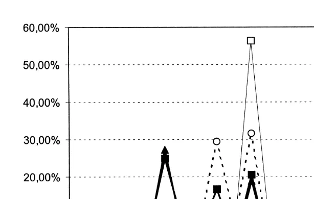
The labor supply disincentives for older workers created by this implicit tax are reflected in the data. Male labor force participation plunges between age 55, when it is almost 90%, to 38% at age 60. It is less than 8% at age 65. Fig. 5 shows that the cross sectional distribution of retirement ages has changed very systematically since 1970. Before the 1972 Reform, the distribution of retirement ages had only one spike. In 1970, age 65 was the retirement age (thin line with hollow square). In 1975, only 2 years after the 1972 Reform became effective, about half of the retirees preferred to retire earlier, and the retirement age distribution had two spikes (dotted line, hollow circles). In 1980, another 5 years later, a three-spike pattern had emerged (thick lines, full square). Since then, there was little change in
3
Fig. 5. Distribution of retirement ages, 1970, 1975, 1980 and 1995. Source: Verband deutscher ¨
Rentenversicherungstrager (VdR), 1997.
this distribution (thick lines, full triangle for 1995). The distribution of retirement ages has its maximum at age 60, the earliest age at which retirement due to health and labor market reasons without formal claims to disability benefits is possible. The other spikes correspond to age 63 for flexible retirement and to age 65 for workers with short work histories. Quite clearly workers take the very first legal opportunity to retire, supposedly because they realize that a postponement inflicts a loss of social security wealth.
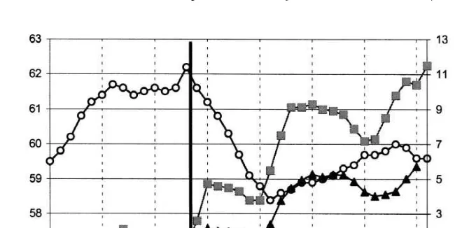
One might argue that the shift in retirement age and the corresponding decline in old-age labor force participation after the 1972 Reform was mainly a demand reaction to rising unemployment rather than a supply response to early retirement incentives. We have two reasons not to believe that this was the case. First, the reform was part of the general expansion of the welfare state after the social democrats took power for the first time in the postwar period. The reform was designed at a time when unemployment was very low while the first steep increase in unemployment (1973 to 1975) happened after the 1972 Reform had already been introduced.
Fig. 6. Average retirement age, 1960–1995. Note: ‘Retirement Age’ is the average age of all new entries into the public pension system. ‘Unemployment rate’ is the general national unemployment rate. ‘Unempl. R. (50–55)’ refers to male unemployed age 50–55. Source: VdR (1997) and BMA (1997).
4
the reform and 1980. After 1980, a positive time-series correlation between retirement age and unemployment is the opposite of what a demand-induced change in old age labor supply would suggest.
Riphahn and Schmidt (1997) confirm this view econometrically. By using panel data that combine regional, sectoral and time variation in unemployment rates and old age labor force participation, they show that the decline in the average retirement age was not a demand response to rising unemployment but rather a supply response to the introduction of early retirement incentives through the 1972 Pension Reform.
4. Pension incentives and retirement age distributions across Europe
The qualitative analysis can be extended to other countries in Europe. In fact, the international variation in old age labor force participation provides another handle to identify disincentive effects of pension systems. The ‘International Social Security Project’ led by Gruber and Wise (1998) compiled comparable social security wealth calculations for a set of European countries plus Japan and the U.S. We use their calculated accrual rates and implicit tax profiles to produce a
4
similar qualitative analysis to the one depicted in Figs. 4 and 5 in the preceding section for the German case.
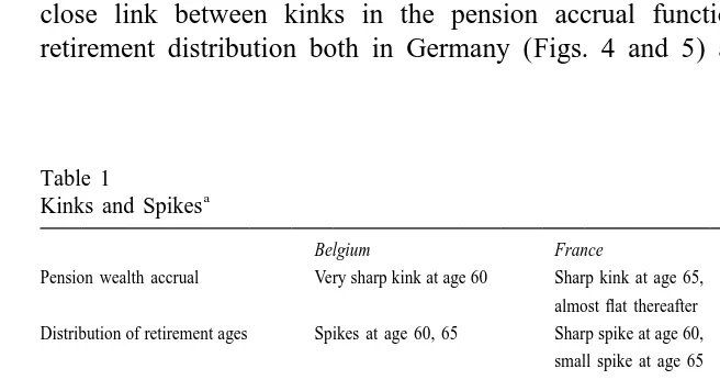
In all countries, labor force exits concentrate at certain ages, creating spikes in the distribution of retirement ages. These spikes can in almost all cases be identified with ages in which certain pension rules start or cease to apply. The most obvious example is the earliest age in which a worker is eligible for social security. In addition, most European pension systems have several ‘pathways’ to retirement, all with different eligibility ages and / or replacement rates, similar to the German example. These rules create kinks in the accrual of social security wealth. Table 1 compiles a list of the kinks in the social security wealth accrual function, and juxtaposes it to the list of spikes in the distribution of retirement ages for seven European countries plus Japan and the U.S. as reference countries. Indeed, the correspondence between kinks and spikes is quite strong.
So far, the evidence on the effects of pension systems on old age labor force participation has been informal. We have accumulated three kinds of qualitative evidence: German workers appear to select the earliest retirement age legally possible (Fig. 5); German workers have responded to the historical experiment of the 1972 Pension Reform is a very consistent way (Figs. 5 and 6); and there is a close link between kinks in the pension accrual function and spikes in the retirement distribution both in Germany (Figs. 4 and 5) and in other countries
Table 1
a Kinks and Spikes
Belgium France Germany
Pension wealth accrual Very sharp kink at age 60 Sharp kink at age 65, Sharp kink at age 60, almost flat thereafter reverse kink at age 65 Distribution of retirement ages Spikes at age 60, 65 Sharp spike at age 60, Sharp spike at age 60, small spike at age 65 small spike at age 65
Italy Netherlands Spain
Pension wealth accrual Negative from age 55, Subsidy at age 59, Sharp kinks at ages 60
kink at age 60 sharp kink at age 60 and 65
Distribution of retirement ages Sharp spikes at ages Very sharp spikes at Small spike at age 60,
55, 60, 65 age 60 sharp spike at age 65
Sweden Japan U.S.
Pension wealth accrual Almost flat until age Sharp kink at age 60 Kinks at age 62 and 65
65 subsidy at 62 and 63
Distribution of retirement Only spike at age 65 Sharp spike at age 60, Spikes at ages 62 and
ages small hump at age 65 65
a
´
Sources: Belgium: Pestieau and Stjins (1998); France: Blanchet and Pele (1998); Germany: ¨
and Siddiqui (1997). We improve on this work by exploiting more systematically the cross-sectional and time-series variation contained in the 1984–1996 German Socio-Economic Panel (GSOEP) that spans several modifications of the German pension system. This section has three parts. We will first describe the data, then the option value framework, and finally our panel data estimation procedure.
5.1. Data
The German Socio-Economic Panel (GSOEP) is an annual panel study of some 5
6000 households and some 15,000 individuals. The design of the GSOEP closely corresponds to the U.S. Panel Study of Income Dynamics (PSID). The panel started in 1984; 13 waves through 1996 are currently available. The GSOEP data provide a detailed account of income and employment status. We constructed an unbalanced panel of all persons aged 55 through 70 in West Germany for which
6
earnings data is available. This panel includes 1639 individuals with 8474 observations. Average observation time is slightly more than 5 years. The panel is left-censored as we include only persons who have worked at least 1 year during our window in order to reconstruct an earning history. There is only little right censoring due to missing interviews. Of the 1639 individuals, 678 have no transitions, 609 have a single transition from employment to retirement, and 352 individuals have more complex histories with at least one reverse transition. Most of these reverse transitions include retirees who pick up part-time work after
7
receiving pension benefits. 35% of our sample persons are female, and the most frequent retirement age is age 60.
5
See Burkhauser (1991) for an English language description. 6
We excluded East Germany because retirement patterns in the East are dominated by the transition ¨
problems to a market economy. See Borsch-Supan and Schmidt (1996) for a comparison. 7
5.2. The option value model
In order to capture the economic incentives provided by the pension system, we employ the option value to postpone retirement (Stock and Wise, 1990). This value expresses for each retirement age the trade-off between retiring now (resulting in a stream of retirement benefits that depends on this retirement age) and keeping all options open for some later retirement date (with associated streams of first labor, then retirement incomes for all possible later retirement ages).
The option value function is closely related to the pension wealth accrual function developed in Section 2 but adds utility from consumption and leisure to the purely financial incentives analyzed in Section 2. Let V (R) denote the expectedt
discounted future utility at age t if the worker retires at age R, specified as follows:
R21 `
a marginal utility of leisure, to be estimated
a probability to survive at least until age s
d discount factor51 /(11r).
Utility from consumption is represented by an isoelastic utility function in
g.
after-tax income, u(Y )5Y Remember that pension income in Germany is effectively untaxed. To capture utility from leisure, utility during retirement is weighted by a .1, where 1 /a is the marginal disutility of work.
The option value for a specific age is defined as the difference between the maximum attainable consumption utility if the worker postpones retirement to some later year minus the utility of consumption that the worker can afford if the worker would retire now. Let R*(t) denote the optimal retirement age if the worker postpones retirement past age t, i.e., max(V (r)) for rt .t. With this notation, the
option value is
*
G(t)5V (R (t))t 2V (t) .t
Since a worker is likely to retire as soon as the utility of the option to postpone retirement becomes smaller than the utility of retiring now, retirement probabilities should depend negatively on the option value.
Estimates for a are between 2.5 and 4 in Germany, see Fig. 7 below. Hence, according to this crude approximation, the tax rates well above 50% exerted by the current public pension system in Germany will lead to early retirement.
We compute the option value for every person in our sample, using the applicable pension regulations and individual earning histories. Additional private pension income is ignored because it represents only a very small proportion of retirement income as described before.
5.3. Econometric estimation method
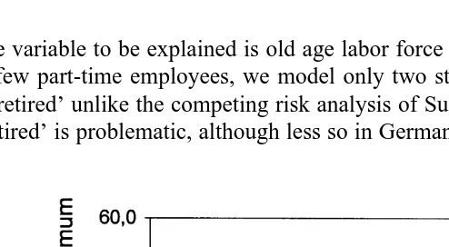
The variable to be explained is old age labor force status. Because Germany has very few part-time employees, we model only two states ‘fully in labor force and fully retired’ unlike the competing risk analysis of Sueyoshi (1989). The definition of ‘retired’ is problematic, although less so in Germany than in other countries (for
Fig. 7. Gridsearch over the inverse marginal disutility of work (a). Note: based on Model 1. 8
the U.S., see Rust, 1990). Retirement definitions commonly employed in the literature include the retirement status self-reported by the respondent, the fact that there are few work hours, or the receipt of retirement benefits, among other definitions. We use the first concept, and include pre-retirement, mainly financed by a mixture of unemployment compensation and severance pay, in our definition of retirement.
Our main explanatory variable is the option value described in the previous subsection. The other explanatory variables are the usual suspects: an array of socio-economic variables such as gender, marital status, wealth (indicator vari-ables of several financial and real wealth categories) and a self-assessed health measure. We do not use the legal disability status as a measure of health since this is endogenous to the retirement decision. The desire for early retirement may prompt workers to seek disability status, and frequently the employer helps in this process to alleviate restructuring. Until recently, disability status was granted for labor market reasons without a link to health.
We link the explanatory variables to the dependent variable by a panel probit model with a parameterized correlation pattern over time. The model can be interpreted as a semi-nonparametric hazard model for multiple spell data, permitting unobserved heterogeneity and state dependence without imposing a
9
functional form on the duration in a given state. Inserting the option value in a regression-type model is a practical estimation procedure that generates robust estimates of the average effects of the option value on retirement, see Lumbsdaine
10 et al. (1992).
Nevertheless, discrete choice models for panel data are necessarily computation-ally involved because the space of possible outcomes is so large, in our case
T
2 58192 choice sequences. Although not all of these choice sequences are observed in our data, there are sufficiently many complex choice sequences in the data to warrant a departure from a simple one-spell hazard model. We structure the choices by cross-sectional utility maximization
Person n chooses retirement in period t⇔unt5Xntb 1 ´ .nt 0
where the utility untis the sum of a deterministic utility component which depends on the vector of observable variables X and a parameter vectornt b to be estimated, and a random utility component ´nt.
We assume that this random component is normally distributed. The probability of a choice sequence is therefore a T-dimensional normal probability. If utilities are correlated over time, which is likely in our panel data, these probabilities are difficult to evaluate. Two examples for intertemporal linkages are particular
9
Flexible hazard rate models of retirement have been estimated by Sueyoshi (1989) and Meghir and ¨ Whitehouse (1997), parametric hazard rate models for German data by Schmidt (1995) and Borsch-Supan and Schmidt (1996).
10
´ 5 u 1hnt n ntwhereh 5 r ?hnt nt211nnt fornnti.i.d. and 0,r ,1.
This model can only be identified in reasonably long panels, and formally if T$3. Classical evaluation of the resulting panel-data probit choice probabilities is computationally infeasible since only random effects can be factorized (Moffitt, 1987) and the number of operations increases exponentially with the length of the panel, T. We instead use the smooth simulated maximum likelihood estimation
¨
(SSML) method proposed by Borsch-Supan and Hajivassiliou (1993) which simulates the choice probabilities by drawing pseudo-random realizations from the underlying error process. This algorithm is very quick, depends continuously on the parametersb and M, and is currently the most efficient method for panel data
11
probit models. This method, as it applies to our application, is sketched in Appendix A.
6. Econometric estimation of disincentive effects: results
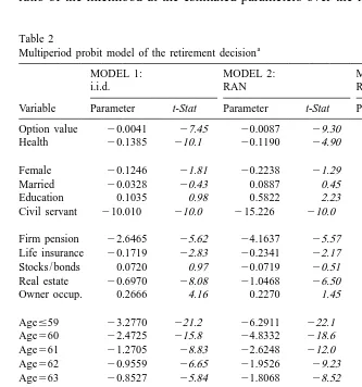
Estimation results are presented in Table 2 below. Dependent variable is labor force status ‘retired’ which includes formal retirement as well as the various forms of pre-retirement. A positive coefficient indicates that the explanatory variables increases the probability of retirement. In addition to the option value, health, and an array of socio-economic variables, we include a full set of age dummies to non-parametrically capture all other unmeasured effects on the retirement decision that are systematically related to age, such as social customs. The reference category is age 65. The parameters ‘hidden’ in the option value,a,g, andd, are set to 3.13, 1.0, and 0.03, respectively. This choice and the (small) sensitivity of the estimated parameters will be discussed below.
We estimate three models. Model 1 has i.i.d. errors. Model 2 corrects for
11
unobserved heterogeneity by a random effect whose standard deviation is reported at the bottom of Table 2. Finally, Model 3 adds an autoregressive error component to Model 2. Estimation results are based on 100 replications. There is no appreciable parameter change if the number of replications is increased, showing that the small sample bias of the SSML estimator has gone away at this number of replications (see Appendix A).
2
Even the simple i.i.d. model fits the data well. The pseudo-R – one minus the ratio of the likelihood at the estimated parameters over the likelihood at zero – is
Table 2
a Multiperiod probit model of the retirement decision
MODEL 1: MODEL 2: MODEL 3:
i.i.d. RAN RAN1AR1
Variable Parameter t-Stat Parameter t-Stat Parameter t-Stat
Option value 20.0041 27.45 20.0087 29.30 20.0096 28.17 Health 20.1385 210.1 20.1190 24.90 20.0991 23.71 Female 20.1246 21.81 20.2238 21.29 20.4172 21.91
Married 20.0328 20.43 0.0887 0.45 0.0337 0.15
Education 0.1035 0.98 0.5822 2.23 0.4303 1.30
Civil servant 210.010 210.0 215.226 210.0 219.777 210.0 Firm pension 22.6465 25.62 24.1637 25.57 24.3530 24.91 Life insurance 20.1719 22.83 20.2341 22.17 20.1781 21.44 Stocks / bonds 0.0720 0.97 20.0719 20.51 20.0776 20.51 Real estate 20.6970 28.08 21.0468 26.50 21.0152 25.55
Owner occup. 0.2666 4.16 0.2270 1.45 0.2441 1.33
Age#59 23.2770 221.2 26.2911 222.1 26.3849 217.1
Age566 0.9891 4.56 1.6842 5.67 1.7242 5.62
Age567 0.6708 3.21 1.3595 4.51 1.3682 4.41
Age$68 0.8810 4.89 1.9073 7.13 1.9398 6.45
Constant 2.2246 13.4 3.3728 10.8 3.4100 9.35
RAN 2.3848 14.8 2.2869 10.3
AR1 0.6903 7.05
Log likelihood 22321.32 21836.91 21744.98
Individuals 8474 1639 1639
Max. periods 1 13 13
Observations 8474 8474 8474
a
coefficients.
Taking account of the intertemporal correlations in the panel appears to be very important. The numerical value of the option value coefficient is severely underestimated in the i.i.d. model which ignores unobserved heterogeneity in the data and autocorrelated disturbances. Comparing the likelihood values between Models 1 and 2, and between Models 2 and 3 reveals that each additional step in the specification of intertemporal linkages is highly significant, and that the full model describes the data best.
The other economic incentives for retirement, the wealth variables, are only partially significant. The GSOEP data does not contain levels of wealth, only indicators whether certain portfolio components ‘firm pension, life insurance, stock and bonds, and real estate’ are present. There are many missing values, here coded as ‘not present’. In general, presence of financial and real wealth decreases the retirement probability. This is not particularly plausible for the presence of a firm pension. However, significant firm pensions are rare in Germany and usually indicate higher valued jobs in which retirement may occur later for reasons not
12 related to the firm pension per se.
The pattern of age dummies reflects the obvious: older workers are more likely retired than younger ones. It is important to measure the option value with the age dummies included in order to purge its estimated coefficient from all other non-economic effects. The omission of age dummies about triples the estimated coefficient of the option value. Most other socio-demographic variables are not significant. The important differences in social security regulations between men and women (women can retire at age 60 if have at least 15 years of retirement insurance history, while men need 35 years to retire at age 63, unless they claim
12
disability) appears to be fully captured by the option value. Marital status and education is also insignificant.
We did not invest a lot of effort to correctly model the retirement subsystem for civil servants. They are actually treated as if they were part of the standard social security system which is not the case. Civil servants are required to work longer than other employees, with a fairly rigid retirement age at 65, although claims to disability are frequent as well as early retirement due to downsizing of the civil service sector. We find a corresponding rather strong negative coefficient, indicating later retirement for civil servants. Excluding the 91 civil servants increases the estimated coefficient of the option value, but not significantly.
Very interesting are the estimated coefficients of the health variable. It is coded 0 for ‘very poor’ to 10 for ‘excellent’. As expected, the coefficients are negative. Less healthy workers retire earlier. In the i.i.d. model, health is more significant than the option value. However, as soon as unobserved population heterogeneity is accounted for, this changes, and the estimated coefficient becomes somewhat smaller. This shows once more the importance to account for intertemporal linkages.
The parameters ‘hidden’ in the option value, namely the inverse marginal disutility of worka, the consumption elasticityg, and the discount rated do not fit in the linear utility framework of the probit model. It turned out that these parameters are very hard to identify simultaneously with b in a nonlinear estimation approach. We therefore adapted a more pragmatic approach. Since a grid search over a yielded a rather flat likelihood with an optimum at 3.13, we used this value for all estimated models (see Fig. 7). This value means that a dollar that has to be earned by work is valued at only about a third of a dollar that is given as a public transfer through the retirement system. This value is somewhat higher than estimates for the U.S. (e.g., Stock and Wise, 1990) but not implausible for Germany with an arguably higher preference for leisure.
The estimated coefficients are rather insensitive to the choice of g in the
g
isoelastic utility function, u(Y )5Y , and to the discount rated. For simplicity, we chooseg 51, effectively identifying consumption with income. Lower values, the more usual case of a declining marginal utility of consumption, increase the coefficient of the option value slightly. The discount factord is assumed to be 3%. Other discount factors in the range between 1 and 6% yield qualitatively similar results.
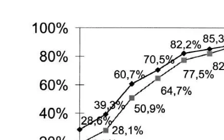
6.1. Simulations
Fig. 8. Actual and predicted cumulative distribution of retirement age. Note: percent retired at given age. Upper graph: current rules (baseline). Lower graph: actuarially fair adjustment factors. Microsimu-lation based on estimated coefficients of Model 3, Table 2.
period through disability or pre-retirement schemes. A shift to an actuarial fair system would cause retirement at ages 59 and below to drop from 28.6% to less than 18.5%.
7. Summary and conclusions
is interesting to note that they have done so before unemployment became widespread in the beginning of the 1980s. Policy-induced early retirement accounts for about a third of early retirement, thus a substantial fraction of total pension expenditures.
The responsiveness of the choice of retirement age to the incentives offered by pension systems has strong policy impacts. The public pension systems do not use retirement-age-dependent adjustments of pension benefits as policy instruments for balancing the budget of the pension system, they even yield incentives to retire early, most frequently at the earliest legal retirement age. While this has alleviated the unemployment problem in the short run, is was an expensive way to do so, and it will hurt in the long run. Rather than awarding later retirement to moderate the labor supply disincentives created by quickly rising social security taxes, social security regulations across the world have encouraged early retirement, thus aggravating the imbalance between the number of workers and pensioners in times of population aging.
The responsiveness to actuarially unfair pension regulations also shows that there is widespread redistribution between from late to early retirees. This increases the deadweight burden generated by contributions to PAYG pension systems, a crucial parameter in computations that try to design welfare-improving transitions from PAYG to fully funded pension systems (e.g., Feldstein and Samwick, 1996; Kotlikoff, 1996). The estimates of the option value model can be used to quantify these order of magnitude for such deadweight burden calcula-tions.
Acknowledgements
I am indebted to Angelika Eymann, Bernd Huber, Mats Persson and Joachim Winter and the participants at the 1998 TAPES conference in Copenhagen, two anonymous referees, and the special editor, Soren Bo Nielsen, for their helpful comments; to Silke Januszewski and Matthias Fengler for their competent research assistance; and to Reinhold Schnabel who provided the earnings history data from the German Socio-Economic Panel. Financial support for this paper was provided by the Deutsche Forschungsgemeinschaft through the Sonderforschungsbereich 504.
Appendix A
In this appendix, we sketch the smooth simulated maximum likelihood (SSML) estimation method as it applies to the application in Section 6.
to draw a T-dimensional vector of unobserved utilities ´t. Let G be the lower diagonal Cholesky factor of the covariance matrix M of the unobserved utility vector´such thatGG 9 5M. We begin by drawing sequentially an auxiliary vector e of T univariate left-truncated normal variates
e5N 0,I s.t. as d #Ge# `,
where a5(a , . . . a ) is now a vector of T truncation points with a1 T t5Xtb. Because G is triangular, the restrictions on e are recursive:
e15N 0,1s d s.t. a1#g11e1# `⇔a /1 g #11 e1# `,
e25N 0,1s d s.t. a2#g21e1l1g22e2# `⇔sa22g21e /1dg #22 e2# `, etc. until t5T.
(A.2)
Hence, each e , tt 51 . . . T, in Eq. (A.2) can be drawn using the univariate formula in Eq. (A.1). Finally, define´5Ge. BecauseGG 9 5M,´has covariance matrix M and is subject to a#Ge# `⇔a#´ # `. Therefore, the probability for a choice sequence i of observation n is, in an expected value sense, the probability that ah jtn
draw of a T-dimensional vector of truncated normal variates er5se , . . . ,er1 rTdfalls in the set of intervals given by Eq. (A.2):
-˜
P (r hitnj) 5Pr a /s 1 g #11 er1# ` ?d Pr[(a22g21 r1e ) /g #22 er 2# `ue ]r1 ? . . . .
5[12F(a /1 g11)]?[12F((a22g21 r1e ) /g22)]? . . . ,
To increase precision, the choice probability is approximated by the average over
R replications:
R
1
˜ ] ˜
P(hitnj)5R
O
P (r himj) .r51
R
Borsch-Supan and Hajivassiliou (1993) prove that P is an unbiased estimator of P. Because the likelihood function depends nonlinearly on the simulated
prob-˜
abilities, L carries a small sample bias that vanishes only if R goes to infinity. In practice, however, are the choice probabilities well approximated already for reasonably small number of replications, independent of the true choice prob-abilities, such that the bias becomes quickly unnoticeable. The table below, referring to the estimates computed for Section 5, Table 2, shows this quite clearly:
a Simulated maximum likelihood parameter estimates by number of replications
Number of 10 20 50 100 200 500 1000
replications
Coefficient of 20.0077 20.0076 20.0089 20.0096 20.0094 20.0095 20.0095 option value
Random effect 1.82 1.96 2.18 2.29 2.26 2.26 2.25
Autocorrelation 0.69 0.69 0.71 0.69 0.70 0.70 0.70 a
See Table 2, Model 3.
Because the generated draws as well as the resulting simulated probabilities depend continuously and differentiably on the parameters b in the truncation vector a and the covariance matrix M, conventional optimization methods can be used to solve the first order conditions for maximizing the simulated likelihood function, and the computational effort in the simulation increases nearly linearly with panel length.
References
´
Blanchet, D., Pele, L.P., 1998. Social Security and Retirement in France. NBER Working Paper No. 6214, Cambridge, MA.
Blundell, R., Johnson, P., 1998. Pensions and Retirement in the United Kingdom. NBER Working Paper No. 6154, Cambridge, MA.
Boldrin, M., Jimenez, S., Peracchi, F., 1998. Social Security and Retirement in Spain. NBER Working Paper No. 6136, Cambridge, MA.
¨
Borsch-Supan, A., 1992. Population aging, social security design, and early retirement. Journal of Institutional and Theoretical Economics 148, 533–557.
¨
Borsch-Supan, A., Hajivassiliou, V., 1993. Smooth unbiased multivariate probability simulators for limited dependent variable models. Journal of Econometrics 58, 347–368.
¨
Geweke, J., 1991. Efficient simulation from the multivariate normal distribution subject to linear inequality constraints and the evaluation of constraint probabilities. In: Computer Science and Statistics: Proceedings of the Twenty-Third Symposium on the Interface, pp. 571–578.
Gruber, J., Wise, D.A. (Eds.), 1998. Social Security and Retirement Around the World. University of Chicago Press, Chicago.
Hajivassiliou, V., McFadden, D., Ruud, P., 1996. Simulation of multivariate normal rectangle probabilities and their derivatives: theoretical and computational results. Journal of Econometrics 72 (2), 85–134.
Kapteyn, A., de Vos, K., 1998. Social Security and Retirement in the Netherlands. NBER Working Paper No. 6135, Cambridge, MA
Kotlikoff, L.J., 1996. Simulating the Privatization of Social Security in General Equilibrium. NBER Working Paper, Cambridge, MA.
Lumbsdaine, R.L., Stock, J.H., Wise, D.A., 1992. Three models of retirement: computational complexity versus predictive validity. In: Wise, D.A. (Ed.), Topics in the Economics of Aging. University of Chicago Press, Chicago, pp. 16–60.
Meghir, C., Whitehouse, E., 1997. Labour market transitions and retirement of men in the UK. Journal of Econometrics 79, 327–354.
Moffitt, T.E., 1987. Life cycle labor supply and social security: a time-series analysis. In: Burtless, G. (Ed.), Work, Health, and Income for the Elderly. Brookings Institution, Washington, D.C. OECD, 1988. Ageing Populations: The Social Policy Implications. OECD, Paris.
Oshio, T., Yashiro, N., 1998. Social Security and Retirement in Japan. NBER Working Paper No. 6156, Cambridge, MA.
Palme, M., Svensson, I., 1998. Social Security and Retirement in Sweden. NBER Working Paper No. 6137, Cambridge, MA.
Pestieau, P., Stjins, J.-P., 1998. Social Security and Retirement in Belgium. NBER Working Paper No. 6169, Cambridge, MA.
¨ Riphahn, R.T., Schmidt, P., 1997. Determinanten des Ruhestandes: Lockt der Ruhestand oder drangt
¨ ¨
der Arbeitsmarkt. Jahrbucher fur Wirtschaftswissenschaften 48 (1), 113–147.
Rust, J., 1990. Behavior of male workers at the end of the life cycle: an empirical analysis of states and controls. In: Wise, D.A. (Ed.), Issues in the Economics of Aging. University of Chicago Press, Chicago.
Rust, J., Phelan, C., 1997. How social security and medicare affect retirement behavior in a world of incomplete markets. Econometrica 65 (4), 781–831.
Schmidt, P., 1995. Die Wahl des Rentenalters-Theoretische und empirische Analyse des Renten-zugangsverhaltens in West- und Ostdeutschland. Lang, Frankfurt.
Stern, S., 1997. Simulation-based estimation. Journal of Economic Literature 35, 2001–2039. Stock, J.H., Wise, D.A., 1990. The pension inducement to retire: an option value analysis. In: Wise,
D.A. (Ed.), Issues in the Economics of Aging. University of Chicago Press, Chicago, pp. 205–230. Sueyoshi, G.T., 1989. Social Security and The Determinants of Full and Partial Retirement: A
Competing Risk Analysis. NBER Working Paper 3113, Cambridge, MA. ¨