STUDY ON THE RETRIEVAL OF SNOW DEPTH FROM FY3B/MWRI
IN THE ATCTIC
Lele Li, Haihua Chen, Lei Guan*
Department of Marine Technology, College of Information Science and Engineering, Ocean University of China, Qingdao, China - (lilele, chh7791, leiguan)@ouc.edu.cn
Commission VIII, WG VIII/6
KEY WORDS: FY3B, MWRI, Sea Ice Concentration, Snow Depth, Brightness Temperature, Radiometer
ABSTRACT:
Snow on sea ice is a sensitive indicator of climate change, it plays an essential role in regulating surface and near surface air temperatures. Given the high albedo and low thermal conductivity, snow is regarded as one of the key reasons for the amplification of the warming in polar regions. The distributions of sea ice and snow depth are essential to the whole thermal conduction in the Arctic. This study focused on the retrieval of snow depth on sea ice from brightness temperatures of the MicroWave Radiometer Imager (MWRI) onboard the FengYun (FY)-3B satellite during the period from December 1, 2010 to April 30, 2011. After cross calibrated to the Advanced Microwave Scanning Radiometer–EOS (AMSR-E) Level 2A data, the MWRI brightness temperatures were applied to calculate the sea ice concentrations based on the Arctic Radiation and Turbulence Interaction Study Sea Ice (ASI) algorithm. According to the proportional relationship between the snow depth and the surface scattering in 18.7 and 36.5 GHz, the snow depths were derived. In order to eliminate the influence of uncertainties in grain sizes of snow as well as sporadic weather effects, the seven-day averaged snow depths were calculated. Then the results were compared with the snow depths from the AMSR-E Level 3 Sea Ice products. The bias of differences between the MWRI and the AMSR-E Level 3 products are ranged between -1.09 and -0.32 cm,while the standard deviations and the correlation coefficients are ranged from 2.47 to 2.88 cm and from 0.78 to 0.90 for different months. As a result, it could be summarized that FY3B/MWRI showed a promising prospect in retrieving snow depth on sea ice.
1. INTRODUCTION
Today the Arctic is an area that attracts intense interest because climate-change signals are expected to be amplified in the region by about 1.5-4.5 times, the high albedo of sea ice and snow depth is postulated as one of the key reasons for the amplification of the warming (Comiso et al., 2014). As the large fraction covering the region, the sea ice and snow on it catch increasingly attentions and become the most important parameters in the Arctic to the global climate system.
As the thermal conductivity of snow is nearly an orders of magnitude smaller than sea ice, the sea ice covered with snow is an effective insulator which limits the energy and momentum exchange between atmosphere and surface. In winter, the thermal flow in the thick ice regions are two orders of magnitude smaller compared to the open water. Even the thin snow will greatly influence the thermal exchange of atmosphere and surface (Comiso et al., 2003). Furthermore, the snow depth is also an important parameter in calculating fresh water budget of sea ice and providing more accurate rainfall estimation.
Nevertheless, due to the particularity of polar environment, the traditional in-situ measurements face great challenges, such as the development of instruments that can provide stable and accurate operation in extremely cold conditions, transport of the instruments and overcoming the influence of the polar night and so on. By contrast the satellite observation has incomparable advantages. It can provide consistent, accurate and integrated data records useful to find the various natural phenomena in polar regions. More and more satellite sensors are used to observe thepolar regions with spectral coverage from visible light to microwave. Comparing to infrared and visible waves, microwave
* Corresponding author
is the most important way to monitor sea ice and snow in polar region for its characteristics of all-day and all-weather observation.
Beginning with the launch of the Electrically Scanning Microwave Radiometer (ESMR) onboard the National Aeronautics and Space Administration of USA (NASA) Nimbus 5 satellite in 1972, which was the first passive microwave sensor successfully applied in the global ice distribution measurement (Gloersen et al.,1974; Parkinson et al., 1987), more and more radiometers were applied to monitor the polar sea ice including the Scanning Multichannel Microwave Radiometer (SMMR) (Zwally et al., 1983; Gloersen et al., 1977) and the Special Sensor Microwave/Imager (SSMI) (Cavalieri et al., 1992; Comiso et al., 1997; Markus et al., 2000).
On May 4, 2002, the Advanced Microwave Scanning Radiometer for Earth Observation System (AMSR-E) was successfully launched aboard the EOS-Aqua satellite. It had significant improvement to sensors before and provided the measurements of terrestrial, oceanic and atmospheric parameters to explore the global water and energy cycles. It also released the operational sea ice products including sea ice concentration, sea ice temperature and snow depth on sea ice. Till October 4, 2011 when the AMSR-E instrument ceased from producing data due to a problem with the rotation of its antenna, it had released the sea ice products more than nine years.
Launched by China Meteorological Administration/National Satellite Meteorological Center (CMA/NSMC), the FY-3 satellites series represent the second generation of Chinese polar-orbiting meteorological satellites with substantively enhanced functionality and technical capabilities. With the capability to provide global, all-weather, multi-spectral, three-dimensional, and accurate observations of atmospheric, oceanic, and land The International Archives of the Photogrammetry, Remote Sensing and Spatial Information Sciences, Volume XLI-B8, 2016
surface states, the FY-3 satellite series can make valuable contributions to improving weather forecasts, natural disaster and environment monitoring of the world. There are two development phases considered for the FY-3 series. The first one is experimental phase from 2008 to 2010 and the second one is the operational service phase beyond 2012. FY-3A and FY-3B are the first batch of FY-3 series launched on May 27, 2008, and November 5, 2010, respectively. They are flown in a circular sun-synchronous near-polar orbit at an altitude of approximately 836 km with an inclination of 98.75° and an orbit period of 101.6 minutes. The satellites are travelling 14.17 orbits during 24 hours and cross the equator in the descending modes at 10:20 a.m. local time for FY-3A and 1:30 a.m. local time for FY-3B. Due to the orbit precession, the FY-3A and FY-3B revisit the same local area in about six days (Yang et al., 2012). There are 11 observation instruments aboard with the spectral range from ultraviolet to microwave, and the data have been provided for uses in numerical weather prediction models and monitoring of the earth’s environments and extreme weather events (Yang et al., 2011; Yang et al., 2011).
The MWRI is one of the 11 sensors mounted on the FY-3B satellite. It scans the earth conically with a viewing angle of 45° and a swath of 1400 km. It is a total power passive radiometer and the observation frequencies are 10.65, 18.7, 23.8, 36.5, and 89 GHz with horizontal and vertical polarizations for each frequency.
At present, there are no on-orbit microwave radiometers that provide operational data of snow depth on sea ice in polar regions, including the MWRI and the Advanced Microwave Scanning Radiometer-2 (AMSR2) which was launched as the successor to AMSR-E on May 18, 2012 aboard the Global Change Observation Mission 1st-Water “SHIZUKU” satellite (GCOM-W1). So it is of utmost importance to develop a snow depth retrieval algorithm based on the brightness temperature of MWRI in the Arctic, and ultimately provide operational products.
2. METHODS
Considering that the in situ data are sufficient to develop a new algorithm, this study focuses on how to derive snow depth from MWRI brightness temperatures using the established algorithm in the Arctic.
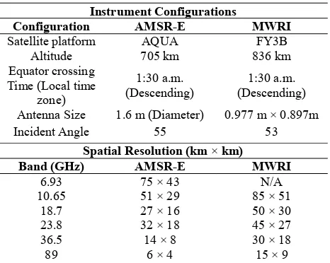
Till now, the most experienced algorithm of snow depth is the AMSR-E algorithm which used to be applied to provide the AMSR-E Level3 sea ice products. Meanwhile the instrument configurations of AMSR-E and MWRI are similar and they also have nearly simultaneous satellite overpass and data acquisition times. As shown in Table 1, except for the calibration system, the channel setting and view geometry of MWRI are almost identical to the AMSR-E (Kawanishi et al., 2003; Yang et al., 2012; Du et al., 2014).
Given these above reasons, the research method of this study was determined, that is, cross calibrating the brightness temperature from MWRI to AMSR-E baseline at first, then calculating the sea ice concentration using ASI (Arctic Radiation and Turbulence Interaction STudy Sea Ice) algorithm and finally deriving the snow depth with the AMSR-E algorithm.
Instrument Configurations
Configuration AMSR-E MWRI
Satellite platform AQUA FY3B
Altitude 705 km 836 km
Equator crossing Time (Local time
zone)
1:30 a.m.
(Descending) (Descending) 1:30 a.m. Antenna Size 1.6 m (Diameter) 0.977 m × 0.897m
Incident Angle 55 53
Spatial Resolution (km × km)
Band (GHz) AMSR-E MWRI Table 1. The main configurations of AMSR-E and MWRI
2.1 ASI algorithm
It is necessary to calculate the sea ice concentrations before retrieving the snow depth. In this study the ASI algorithm was utilized to calculate the sea ice concentration. It is based on the theory that the polarization difference of the emissivity near 90 GHz is similar for all ice types and much smaller than for open water. This is also true for the polarization difference of brightness temperature. It can be assumed that the sea ice concentration is functions of polarization difference as the Eq. (1) shows:
C = P + P + P + (1) where c= sea ice concentration
p = polarization difference of brightness temperature at 89 GHz
to = the coefficients of the equation
After a series of physical and mathematical derivation, the coefficients are deduced (Spreen et al., 2008).
As the conspicuous influence of atmospheric cloud liquid water and water vapour on the brightness temperatures at 89 GHz, using thetwo channels to calculate the sea ice concentrations has a pronounced disadvantage. In order to eliminate spurious weather effects over the open ocean, two weather filters are applied respectively.
The first one utilizes GR(36.5V/18.7V) meaning the gradient ratio of the 36.5 and 18.7 GHz channels (Gloersen and Cavalieri, 1986) which is positive for open water but near zero or negative for ice. This ratio mainly filters the cases with high cloud liquid water. The GR is defined as:
GR(36.5V/18.7V) =[ ( . )[ ( . ) ( . )]( . )] (2) Where 36.5V = the vertical channel at 36.5 Ghz
(36.5V) = the brightness temperatures of 36.5V channel
Additionally, to exclude the cases of high water vapour above open water, the GR(23.8V/18.7V) is used (Cavalieri et al., 1995).
The thresholds of the two GR are set to 0.045 and 0.04, respectively. Through the process above, all ice concentrations The International Archives of the Photogrammetry, Remote Sensing and Spatial Information Sciences, Volume XLI-B8, 2016
can be kept above 15% which is defined as the ice edge contour line in general (Gloersen et al., 1992; Spreen et al., 2008).
2.2 Snow depth algorithm
The AMSR-E algorithm was initially developed through the comparison of in situ snow depth measurements with the SSM/I brightness temperatures of Southern Ocean sea ice (Markus et al., 1998), and then was applied to the first-year sea ice regions in the Arctic.
The main idea of the algorithm is similar to the AMSR-E snow-on-land algorithm (Kelly et al., 2003), utilizing the assumptions that scattering increases with increasing snow depth and the scattering efficiency is greater at 37 GHz than at 19 GHz. For snow-free sea ice, the gradient ratio is near zero and it becomes more and more negative as the snow depth increases.
According to the proportional relationship between the snow depth and the surface scattering, the GR of 36.5 and 18.7 GHz on vertical channels are used to regress the snow depth on sea ice (Comiso et al., 2003).
T = the average values of brightness temperatures on different channels for open water
The algorithm has some limitations: 1) The algorithm is applicable to dry snow only, since in case of wet snow, the emissivity of 18.7 GHz and 36.5 GHz are basically consistent and the snow depth could not be determined by GR (36.5/18.7). 2) As the penetration depth of the microwave signals at 36.5 and 18.7 GHz is less than 50cm, the snow depth on sea ice can be calculated only under the limit of 50 cm. 3) because of the similarity between the multiyear sea ice and the deep snow, the algorithm is only valid for seasonal ice areas.
3. DATA
In addition to the two algorithms above, the study presented is based on three data sets. they are the brightness temperatures from MWRI and AMSR-E, the snow depths as the validation data from the AMSR-E Level 3 standard sea ice products.
3.1 Brightness temperature
The NSMC archives and distributes 3 level products of the MWRI, including MWRI Level 1 swath brightness temperature records, Level 2 terrestrial, oceanic and atmospheric parameters records and Level 3 terrestrial and oceanic parameters records. (Yang et al., 2012).
The level 1 brightness temperature records utilized in this study are stored in the form of orbital swath records with 28 separated ascending and descending files one day. Every file contains 10 channels records in original resolutions at 5 frequencies with dual polarizations.
In this study, the brightness temperature data of vertical channels at 18.7, 23.8 and 36.5 GHz, both the vertical and horizontal channels at 89 GHz were applied to calculate the snow depth on sea ice in the Arctic. The space coverage is the north of 30°N and the time coverage is from December 1, 2010 to April 30, 2011 considering the overlap period of MWRI and AMSR-E.
3.2 Validation data
The AMSR-E Level 3 standard sea ice products were utilized to examine the performance of the results. As presented above the NSIDC provides this data set which includes parameters of sea ice concentration generated using the enhanced NASA Team (NT2) algorithm (Markus et al., 2000), sea ice temperature, and snow depth on sea ice by AMSR-E algorithm. These products together with AMSR-E calibrated brightness temperatures are mapped to a standard polar stereographic grid with the spatial resolution of 12.5 km (Markus et al., 2008; Cavalieri et al., 2014). In this study the space coverage is the Arctic and the time range is from December 1, 2010 to April 30, 2011.
4. PROCEDURE AND RESULTS 4.1 Procedure
Retrieval of the snow depth from brightness temperatures of the MWRI was divided into four steps in this study.
4.1.1 Cross calibration: The first step was to cross calibrate the brightness temperature data from MWRI to the AMSR-E baseline. Considering the overpass time of the two sensors, five-month orbital swath brightness temperature records from December 1, 2010 to April 30, 2011 were extracted over the Arctic areas. The linear equation is used as the calibration formula. After elimination of the invalid data, there were approximately 50 million matchup data on each channel which were used to obtain the calibration coefficients.
4.1.2 Calculating sea ice concentration: In this step, the cross calibrated brightness temperatures were input into the ASI algorithm. The coefficients used in this work are 1.64 × 10 , -0.0016, 0.0192 and 0.9710. After weather filter by two GRs, the sea ice concentrations were projected to the polar stereographic projection grids with a spatial resolution of 12.5 km. Then the daily sea ice products averaged from orbit records were outputted.
4.1.3 Retrieving snow depth on sea ice: Based on the daily sea ice concentrations and the brightness temperatures on 18.7V and 36.5V channels, daily snow depths were calculated using the AMSR-E algorithm in the Arctic.
4.1.4 Average snow depth of seven-day: Due to that the snow melted during daytime are usually to freeze at night, the grain sizes become bigger. This process will cause that the surface emissivity decrease much faster at 36.5 GHz than at 18.7 GHz and may overestimate the snow depth. In order to eliminate the influence of uncertainties in grain sizes and density variations as well as sporadic weather effects, like the five-day average snow depth of the AMSR-E Level 3 products, the data retrieved in this study were averaged to seven-day records.
In this step, the multiyear sea ice points were marked based on a threshold of GR (36.5V/18.7V), while the variability and snow melt points based on the change of snow depth in seven days. The International Archives of the Photogrammetry, Remote Sensing and Spatial Information Sciences, Volume XLI-B8, 2016
4.2 Results
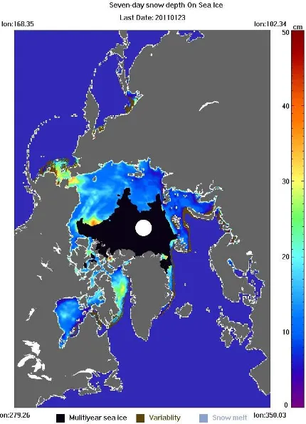
From the process above, the sea ice concentrations and the seven-day averaged snow depths were derived. Fig. 2 and Fig.3 show the sea ice concentrations and the snow depths on January 23, 2011 as a representative.
Figure 2. The sea ice concentration of MWRI on January 23, 2011
Figure 3. The snow depth of MWRI on January 23, 2011
5. VALIDATION
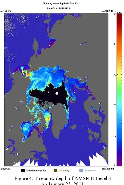
As presented above, the snow depth from AMSR-E Level 3 products were applied to evaluate the results. In order to compare with the results, the snow depth from AMSR-E Level 3 products on January 23, 2011 is shown in Fig. 4.
Figure 4. The snow depth of AMSR-E Level 3 on January 23, 2011
Comparing Fig. 3 and Fig.4, it can be concluded that the results have a relative consistency with the AMSR-E Level 3 products in the Arctic.
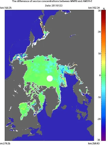
To view the differences more intuitively, the difference values are shown in Fig. 5 which were calculated only at non-flag points.
Figure 5. MWRI minus AMSR-E Level 3 on January 23, 2011
In order to display the statistics of the differences, the discrepancies between this study and the AMSR-E Level 3 products for each month are provided in Table 6. it demonstrates that the snow depth from this study is generally lower than the AMSR-E Level 3 products in the Arctic. The biases of the differences are ranged between -1.09 and -0.32 cm,while the standard deviations and the correlation coefficients are from 2.47 to 2.88 cm and from 0.78 to 0.90, respectively. The differences are basically consistent in different months.
Month Number Bias /cm STD /cm correlation coefficient Dec. 2010
Jan. 2011 Feb. 2011 Mar. 2011 Apr. 2011
841 923 1 008 835 1 000 937 1 091 325 1 091 112
-0.32 -1.09 -0.93 -0.64 -1.04
2.79 2.57 2.47 2.88 2.79
0.797 0.876 0.850 0.862 0.902 Table 6. Statistics of the snow depth differences from this study
and the AMSR-E L3 products
Moreover, the histogram of the differences in January 2011 were drawn as an example to illustrate the distribution of the differences in Fig. 7. It shows that the differences between the two data sets are basically symmetrical distributed with a centre of -2 to 0 cm which are consistent with the statistics above. The International Archives of the Photogrammetry, Remote Sensing and Spatial Information Sciences, Volume XLI-B8, 2016
Figure 7. The histogram of the snow depth differences in January 2011
Accounting for the discrepancies between the results of this study and the AMSR-E Level 3 products, the sea ice concentration differences are considered as the main contributor. The algorithm applied to this study is the ASI algorithm, while the AMSR-E Level 3 products are derived from the NT2 algorithm. According to (Brucker,2013), 5% variation in sea ice concentration will cause variations of the snow depth about 1 to 6 cm. the discrepancies of the sea ice concentrations retrieved from the two algorithms on January 23, 2011 are shown in Fig. 8. Time was selected here to keep the consistency with above.
Figure 8. The sea ice concentrations from ASI minus that from NT2 on January 23, 2011
Comparing to Fig. 5 and Fig. 8, it can be seen that where the difference of the snow depth is the biggest, the difference of sea ice concentration is also the largest. And a conclusion can be drawn that the greater the difference of sea ice concentrations, the greater the difference of the snow depths.
The second contributor of the differences is considered to be the deviation from the algorithm coefficients. The AMSR-E algorithm is based on the SSMI data and after cross calibration from AMSR-E to SSMI, the same regression coefficients are
applied to the AMSR-E brightness temperature, and to MWRI now, it may bring additional errors.
And the third one is from the brightness temperatures. Although the brightness temperatures from MWRI were calibrated to AMSR-E, the two data sets still have the deviations. So the snow depths retrieved from them will have differences.
According to the validations above, it is proved that the method taken in this study is feasible and the results are reasonable.
6. VARIATION
Meanwhile, in order to observe the changes of snow depth in the Arctic, 4 points were selected from different seas to analyze the trends from December 1, 2010 to April 30, 2011. The positions of the points are presented in Fig. 9.
Figure 9. Positions of the selected points
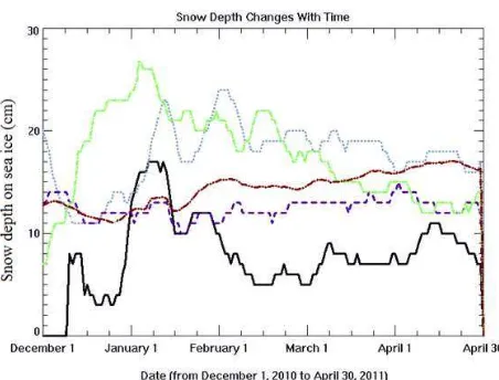
The plots of the snow depth at 4 points accompanied with the averaged snow depth in the arctic were drawn in Fig. 10. It illustrates that for point 1, the peak of the snow depth appeared in January, and the values are smoother at the rest of the time. Similarly, snow depth of point 2 and point 4 reached the peak at January and declined smoothly later. While point 3 shows a different trend that was generally smooth during the whole period. But for the whole Arctic, the average snow depth increases smoothly and reaches the highest in mid April.
Figure 10. Variations of snow depth at 4 points (black Solid: point 1; dotted: point 2; dashed: point 3; dash dot: point 4; red
line: average snow depth of the Arctic)
7. CONCLUSION
In this study, based on the snow depth on sea ice algorithm of AMSR-E and the ASI sea ice algorithm, the cross calculated brightness temperatures from MWRI to AMSR-E baseline were utilized to retrieve the sea ice concentration and the snow depth on sea ice in the Arctic. Comparison of the results with the snow depth of the AMSR-E Level 3 sea ice products it turns out that the two data sets are basically consistent with a bias ranged between -1.09 and -0.32 cm and correlation coefficients ranged between 0.78 and 0.90 for different months. After validation, it can be concluded that the method in this study can be used to retrieve the snow depth on sea ice from MWRI brightness temperatures in the Arctic and it shows a promising prospect.
ACKNOWLEDGEMENTS
This work was supported by the Global Change Research Program of China (2015CB953901). The FY-3B/MWRI TBs products used for this study were provided courtesy by the NSMC FengYun Satellite Data Center. The Aqua/AMSR-E Level 3 Sea Ice products were provided courtesy by the NSIDC.
REFERENCES
Ashcroft, P., Wentz F., 2013. AMSR-E/Aqua L2A global swath spatially-resampled brightness temperatures, Version 3. NASA National Snow and Ice Data Center Distributed Active Archive
Center, Boulder, Colorado, USA.
http://dx.doi.org/10.5067/AMSR-E/AE_L2A.003
Cavalieri D. J., Comiso J. C., Markus T., 2014. AMSR-E/Aqua Daily L3 12.5 km Brightness Temperature, Sea Ice Concentration, & Snow Depth Polar Grids, Version 3. NASA National Snow and Ice Data Center Distributed Active Archive Center, Boulder, Colorado, USA. http://dx.doi.org/10.5067/AMSR-E/AE_SI12.003
Cavalieri D. J., Crawford J., Drinkwater M., Emery W. J., Eppler D. T., Farmer L. D., Goodberlet M., Jentz R., Milman A., Morris C., Onstott R., Schweiger A., Shuchman R., Steffen K., Swift C. T., Wackerman C., Weaver R. L., 1992. NASA sea ice validation program for the DMSP SSMI: Final report. NASA Technical Memorandum 104559. National Aeronautics and Space Administration, Washington, D.C., USA.
Cavalieri, D. J., Germain K. M. S., Swift C. T., 1995. Reduction of weather effects in the calculation of sea-ice concentration with DMSP SSM/I. Journal of Glaciology, 41(139), pp. 455–464.
Comiso J. C., Cavalieri D. J., Markus T, 2003. Sea ice concentration, ice temperature, and snow depth using AMSR-E data. IEEE Transactions on Geoscience and Remote Sensing, 41(2), pp. 243-252.
Comiso J. C., Cavalieri D. J., Parkinson C. L., Gloersen P., 1997. Passive microwave algorithms for sea ice concentration - a comparison of two techniques. Remote Sensing of Environment, 60(3), pp. 357–384.
Comiso J. C., Hall D. K., 2014. Climate trends in the Arctic as observed from space. WIREs Clim. Change, 5, pp. 389-409.
Du J. Y., Kimball J. S., Shi J. C., Jones L. A., Wu S. L., Sun R. J., Yang H., 2014. Inter-calibration of satellite passive microwave land observations from AMSR-E and AMSR2 using overlapping FY3B-MWRI sensor measurements. Remote
Sensing, 6(9), pp. 8594-8616.
Gloersen P., Barath F. T., 1977. A scanning multichannel microwave radiometer for Nimbus-G and SeaSat-A. IEEE
Journal of Oceanic Engineering, 2(2), pp. 172–178.
Gloersen P., Campbell W. J., Cavalieri D. J., Comiso J. C., Parkinson C. L., Zwally H. J., 1992. Arctic and Antarctic sea ice, 1978–1987: satellite passive microwave observations and analysis. Annals of Glaciology, NASA Spec. Publ., 511, pp. 290.
Gloersen, P., Cavalieri D.J., 1986. Reduction of weather effects in the calculation of sea ice concentration from microwave radiances. Journal of Geophysical Research, 91(C3), pp. 3913-3919.
Gloersen P., Willicit T. T., Chang T. C., Nordberg W., Campbell W. J., 1974. Microwave maps of the polar ice of the Earth.
Bulletin of the American Meteorological Society., 55, pp. 1442–
1448.
Holland M. M., Bitz C. M., 2003. Polar amplification of climate change in coupled models. Climate Dynamics, 21(3-4), pp. 221– 232.
Kawanishi T. J., Sezai T., Ito Y., Imaoka K., Takeshima T., Ishido Y., Shibata A., Miura M., Inahata H., Spencer R. W., 2003.The Advanced Scanning Microwave Radiometer for the Earth Observing System (AMSR-E): NASDA’s contribution to the EOS for global energy and water cycle studies. IEEE
Transactions on Geoscience and Remote Sensing, 41(2), pp.
184–194.
Kelly R., Chang A. T. C., Tsang L., Foster J. L., 2003. A prototype AMSR-E global snow area and snow depth algorithm.
IEEE Transactions on Geoscience and Remote Sensing, 41(2),
pp. 230-242.
Markus T., Cavalieri D. J., 1998. Snow depth distribution over sea ice in the Southern Ocean from satellite passive microwave data. In: Antarctic Sea Ice: Physical Processes, Interactions and
Variability, Antarctic Research Series, Vol. 74, pp. 19–40.
Markus T., Cavalieri D. J., 2000. An enhancement of the NASA team sea ice algorithm. IEEE Transactions on Geoscience and
Remote Sensing, 38(3), pp. 1387–1398.
Markus T., Cavalieri D. J., 2008. AMSR-E algorithm theoretical basis document supplement: sea ice products. Hydrospheric and Biospheric Sciences Laboratory, NASA Goddard Space Flight Center, Greenbelt, MD, USA.
Parkinson C. L., Comiso J., Zwally H. J., Cavalieri D. J., Gloersen P., Campbell W. J., 1987. Arctic sea ice, 1973–1976: satellite passive microwave observations. In: Annals of
Glaciology: NASA Spec Publ, 489, pp. 296.
Spreen G., Kaleschke L., Heygster G., 2008. Sea ice remote sensing using AMSR-E 89-GHz channels. Journal of
Geophysical Research, 113(113),pp. 447-453.
Worby A. P., Markus T., Steer A. D., Lytle V. I., Massom R. A., 2008. Evaluation of AMSR-E snow depth product over East Antarctic sea ice using in situ measurements and aerial photography, Journal of Geophysical Research, 113(C5), pp. 1202-1215.
Yang H., Lv L. Q., Xu H. X., He J. K., Wu S. L., 2011. Evaluation of FY3B-MWRi instrument on-orbit calibration accuracy. In:
Archives of IEEE International Geoscience and Remote
Symposium, Vancouver, Canada, 24(8), pp. 2252-2254.
Yang H., Weng F. Z., Lv L. Q., Lu N. M., Liu G. F., Bai M., Qian Q. Y., He J. K., Xu H. X., 2011. The fengyun-3 microwave radiation imager on-orbit verification. IEEE Transactions on
Geoscience and Remote Sensing, 39(11), pp. 4552-4560.
Yang H., Zou X., Li X., You R., 2012. Environmental data records from FengYun-3B microwave radiation imager. IEEE
Transactions on Geoscience and Remote Sensing, 50(12), pp.
4986-4993.
Yang J., Dong C. H., 2010. A new generation of FY polar orbit meteorological satellite products and applications. Beijing, Science Press.
Zwally H. J., Comiso J.C., Parkinson C. L., Campbell W. J., Carsey F. D., Gloersen P., 1983. Antarctic sea ice, 1973–1976: satellite passive-microwave observations. Annals of Glaciology, NASA Spec. Publ., 459, pp.1983.