OFF-LINE VS. ON-LINE CALIBRATION OF A PANORAMIC-BASED MOBILE
MAPPING SYSTEM
Bertrand Cannelle,Nicolas Paparoditis,Marc Pierrot-Deseilligny,Jean-Pierre Papelard
IGN, MATIS
73 Avenue de Paris, 94160 Saint-Mand´e, France; Universit´e Paris-Est
KEY WORDS:mobile mapping system, photogrammetry, multi-camera panoramic head, calibration, off-line calibration, on-line calibration, panoramic head calibration with very low image overlap, bundle adjustment.
ABSTRACT:
This paper presents two methods to calibrate a photogrammetric-based mobile mapping system.
The paper is organised as follow. The first part presents the problem we are trying to solve, i.e. the calibration of multi-camera head on a mobile mapping system equipped with an Inertial Navigation System (INS). We want to estimate on the one hand the relative pose of images within the head and on the other hand the relative pose between the head and the INS The second part presents the first calibration method which is based on observations of a sub-millimeter accuracy topometric target network. The third part explores a method to determine the calibration on-line, i.e. using the images acquired during the surveys. The final section compare the two methods on an neutral data set and resumes the pros and cons of each method.
1 INTRODUCTION
Mobile mapping systems have encoutered a large success in the recent years with wide applications ranging from 3D metrology to multimedia as evidenced by the work of (Ellum and El-Sheimy, 2002) or even more recently in (Petrie, 2010). Most of these systems are LiDAR-based for metrology and inventory for road-based applications. Nevertheless some other systems uses optical devices for surveying. Some use stereo-rigs in order to provide 3D photogrammetric plotting services or to ease automatic 2D or 3D object extraction from images. Some other systems such as the Google and the EarthMine cars are panoramic-based in order to propose immersive visualisation possibilities often on the web. Nevertheless, images are not used so much yet for 3D metrol-ogy. For the applications, where the accuracy of the 3D maps or 3D object-based databases generated from the optical imagery are crucial, e.g. 3D surveying for civil engineering and 3D maps or 3D visual landmarks databases for autonomous navigation, an accurate geometric calibration of the system is mandatory. In order to achieve such a calibration, one needs to master on the one hand internal geometric calibration of all sensors, and on the other hand the relative pose estimation of all sensors with one the other and the relative pose of the set of sensors with respect to the reference frame of the vehicle they are mounted on.
In this paper we aim at calibrating a multi-camera panoramic head on a vehicle, i.e. to determine the relative orientation of all cameras composing the panoramic head with respect to the vehi-cle. Our panoramic head can not be calibrated as a whole by itself due to the fact that the the overlapp between the images is very small (a few pixels). We will thus aim at estimating independtly the extrinsic parameters of each camera composing the camera. We will describe and compare two complete calibration processes to estimate the pose of cameras (composing a panoramic head) relatively to the vehicle they are mounted on. The first, called the off-line calibration, is carried out independtly from the surveys and needs a topometric target network and a manual and/or auto-matic plotting of target observations in the images. The second, called the on-line calibration, is carried out directly on the survey data. Both methods will be compared.
2 DESCRIPTION OF OUR MOBILE-MAPPING VEHICLE
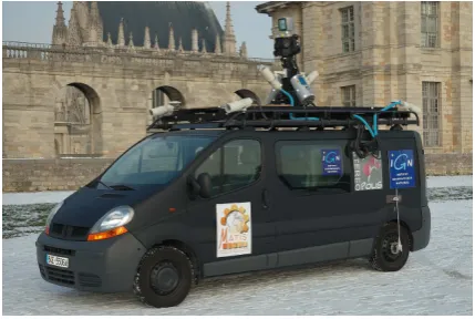
In this section and in Figure 1, we present our photogrammetric-based Mobile Mapping Sytem St´er´eopolis V2.
Figure 1: St´er´eopolis V2
2.1 The panoramic head
Our panoramic head is based on a set of 10 full HD PIKE cameras with high quality lenses (no chromatic aberrations on the image field). These scientific cameras are higly synchronisable, i.e. all images captured within a panoramic are acquired at the same time thus avoiding parallax problems. These cameras have also with very high dynamics (close to 12 bits) to capture imagery with all lighting conditions (from hard shadows to bright sun exposures). All the cameras of the head acquire images at the same aperture for each pose and all along the survey. Moreover, the exposure time is small to avoid blur due to the vehicle displacement. The images which are captured have a very high angular resolution, i.e. 1 pixel correesponds to 0.04 degrees.
of the perspective centers corresponding the CAD design plans. The perspective center is the position where all perspective beams converge and is very difficult to estimate in theory as it does not correspond to one unique point in reality in a complex optics (Mc-Glone et al., 2004). We thus measure the position of the entry nodal point assumed to be equal to the perspective center with re-spect to object space with a well-known ad-hoc optical alignment technique. The idea is to put the camera on a pan-tilt system and to capture series of photos with near and far objects by pan-tilting the camera. If the relative order between the objects changes be-tween the images, the camera is not well centered and the camera body is shifted manually until convergence.
2.2 The positioning system
An inertial Navigation System hybridating, in a tightly-coupled way, the data of two GPS, an Inertial Measurement Unit (IMU), and an odometer provides the position and an accurate orienta-tion of the vehicle in a global reference system even when GPS is masked or corrupted by multiple paths. During GPS gaps, the absolute position reconstructed from the IMU only is biased due to its drifts. The trajectography data acquired on-line by the INS is processed a posteriori in both forward and reverse directions to smooth trajectory and reduces the errors due to lacks of GPS signal. The IMU is mounted rigidely at the foot of the panoramic multi-head camera in order to avoid level arm errors (the wider the level arm, the higher the impact on position and rotation er-rors).
22 23 21
33 32
31 34
41
42 43
a b
Figure 2: (a) Panoramic head mounted on mobile mapping sys-tem. (b) Id of cameras used
For orientations, we can not use the CAD design plan as a ref-erence. Indeed on the one hand the optical axis of each camera is different and on the other the impact of a mechanical errors is non negligible. For example, for a 4 cm camera body size, a 0.1 mm drilling error on the camera fixation holes induce an error of 2.5 pixels on the center of the images and 8 on the border of the images. Nevertheless, these CAD orientions can be used as initial solutions for the linearisation of the bundle equations.
3 CALIBRATION ON A TOPOMETRIC TARGET NETWORK
This section first introduces the conventions and systems of coor-dinates used throughout the paper. Then, the calibration process of the mobile mapping system is detailed. Finally experimenta-tions are presented.
In this part, almost figures contains 3D model. They serve only for illustrations but are not used as input to process.
3.1 Notations and Conventions
Integrating sensors to a mobile platform requires to define several coordinate systems:
Sste
Rste,cam
Tgrd,ste
Rgrd,ste
. Mgrd
Figure 3: Systems of coordinates used
• Ground reference system (grd)
• Reference system of the mobile mapping system (ste) de-fined by a rotationRgrd,ste and a translationTgrd,ste in
ground coordinates
• Reference system of a camera (cam) defined by a rotation Rste,camand a translationTste,cam.
Figure 3 represents theses different systems. If we callMxxx
the coordinates of a pointM in thexxxcoordinate system, the change of coordinates are expressed as:
Mste=Rgrd,ste(Mgrd− Tgrd,ste) (1)
Msen=Rste,cam(Mste− Tste,cam) (2)
In ”classical” photogrammetry (McGlone et al., 2004), a 3D point Mgrdin object space projects itself in the image space of a
cam-era with coordinates(c, l)by:
c l
=
cP P A
lP P A
−ptRgrd,cam(Mgrd−Sgrd) kRgrd,cam(Mgrd−Sgrd)
(3)
where:
• p: the focal lenght of the camera
• (cP P A, lP P A): the principal point of auto collimation in
image space
• kthe third unitary vector of the ground system coordinate • Sgrdthe position of the center of the camera in the object
space andRgrd,camthe rotation of the camera with the
ob-ject space.
Equations (1), (2) and (3) can finally be combined to build (4), which is formula to obtain the image measurement in camera i of a pointMin the ground reference frame.
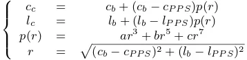
Unlike the approch of (Scheller et al., 2007) who calibrates at the same time the intrinsic and extrinsic parameters, we choose to calibrate each camera separately following a process similar to (Tsai, 1987) and (Hartley and Zisserman, 2000). We consider a radial polynomial distortion model of the form:
cc = cb+ (cb−cP P S)p(r)
lc = lb+ (lb−lP P S)p(r)
p(r) = ar3
+br5
+cr7
r = p
(cb−cP P S)2+ (lb−lP P S)2
where(cb, lb)is the measure taken directly in image space and
(cc, lc)is the corrected measurement. Note that the Principal Point of Symmetry(cP P S, lP P S)which is the intersection of the
c l
i,j
=
cP P A
lP P A
i
−pi
Rstej,camiRgrd,stej Mgrd− Rcami,stejScami+Tstej,grd
tkR
stej,camiRgrd,stej Mgrd− Rcami,stejScami+Tstej,grd
=fi,j(Mgrd) (4)
3.2 Calibration process
One can see in formula 4 that both positions and orientations intervene. To initialize our photogrammetric bundle we use as initial solutions the orientations and positions of cameras corre-sponding to the CAD design of the vehicle. In the compensation we only allow positions of the perspective centers to be very close to the ones of the design (one to a few centimeters). Using these strong observations are important as the positions can not be de-termined as precisely by the bundle adjustment itself. The orien-tation interval is set much looser as the orienorien-tation of the optical axis of each camera depends on the quality of the alignment of the lenses and on the mechanical alignment of the optics on the camera body.
3.3 Calibration on a surveyed 3D target network
We have show a topometry method to determine with precision the position of the camera but we have demonstrated it’s difficult to determine the rotation. Now a method will be presented to find the best positions and rotations of the camera. This is a method on a topometric target network which needs an adapted place.
Our target network is a facility where the mobile mapping sys-tem can move and capture images of 3D surveyed targets. These targets are measured with a sub-millimeter accuracy with precise surveying techniques. The observation of the 3D targets in the images is carried out manually by an operator (but this could also be made automatically with specific coded targets).
Figure 4 presents four positions of St´er´eopolis V2 with the multi-camera images which have been acquired and the 3D rays corre-sponding to the image observations of targets.
a b
Figure 4: (a) Representation of St´er´eopolis V2 during calibration phase. Image plans (in transparent) and measurements(lines) are also visible. (b) Example of target
3.4 Mathematical formulation of the problem
In formula 4, the equation explains the link between points in the ground reference system and corresponding measurements in im-age space. So with a set of Ground Control Points (GCP) (noted Mgrdin equation), and corresponding image measurements, we
propose to calibrate our system using a method similar to the bun-dle adjustment presented in (Schmid, 1959) and (Triggs et al., 2000) and used by (Scheller et al., 2007) in the mobile mapping calibration context. Formula 5 presents the system to minimize which is solved by least squares and bundle adjustment. To ini-tialize the system, we useTgrd,ste, Rgrd,ste with information given by positionning system andScam,Rste,camwith CAD
arg min [Scam,R
ste,cam] #N c i=1
h
T
grd,ste,Rgrd,ste
i#N p j=1
N m
X
k N c
X
i N p
X
j
fi,j−
ck
lk
i,j
!2 (5)
with :
• N mis the number of image measurments.
• N cis the number of camera on the mobile mapping vehicle.
• N pis the number of position of the mobile mapping vehicle.
• T(c, l)i,jis the measurekin image taken by cameraiin the posejof the MMS.
3.5 Experimentations
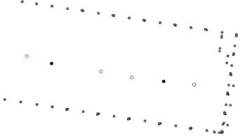
We have choose 4 positions of the vehicle to calibrate the sys-tem. We have manually measured 534 target projections in the different images. Figure 5 presents a bird’s view of the geometric configuration of our experimentation.
Figure 5: Configuration and distribution of image poses and tar-gets. In gray: point known in 3D, in white: position of the vehi-cle used for calibration, in black: position of the vehivehi-cle used for control.
3.5.1 Quantitative results On table 1, we can see the differ-ence between with no calibration and with calibration. Histogram on figure 6 describes the repartition of norm of measurements as a function of residuals. Most of image residues smaller than 1 pixel. Mean is 0.47 pixels and standard deviation is 0.37 pixels. By contruction,the sum of the residues of images measurments is null. We all observe that the sum of residues per camera is also null whichs proves there is no biais in the estomation.
res. (pix.) ♯meas.
10.0 20.0 30.0 40.0 50.0 60.0 70.0 80.0
0 0.5 1 1.5 2 2.5 3
Cameras Before Calib. (pix.) After Calib. (pix.) mean std. dev. mean std. dev.
21 6.10 1.31 0.41 0.25
22 3.47 1.99 0.76 0.41
23 7.52 3.63 0.43 0.25
31 18.67 2.50 0.25 0.14
32 15.27 1.79 0.57 0.39
33 8.16 2.02 0.35 0.22
34 22.12 1.91 0.44 0.25
41 6.00 2.24 0.49 0.31
42 2.21 1.09 0.35 0.22
43 5.00 0.89 0.41 0.19
Table 1: Norm of residues on images measurements per cameras before and after calibration. std. dev. (standart deviation).
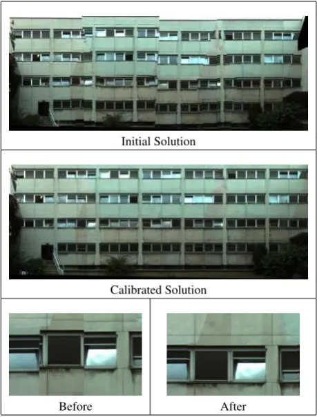
3.5.2 Qualitative results On figure 7 one can see one of the (surveyed) facades of the facility textured with the images ac-quired by our MMS. The images are projected on the 3D plane of the facade which is in the same reference system as the tar-gets. Before calibration, windows are not aligned, and windows edges are discontinuous on each side of the mosaicquing. After calibration windows are aligned and egdes are perfectly continu-ous. This means that the relative pose of the cameras are correctly estimated.
Initial Solution
Calibrated Solution
Before After
Figure 7: Comparison of reprojection of images on plan before and after calibration
3.5.3 Control To control the result of the calibration, we used on the same facility two extra poses of the MMS with 188 mea-surements on the images. We only estimate the pose of the vehi-cle by bundle adjustment and we use as position and rotation of cameras the results of process presented in 3.2. Only 3 targets are used as GCPs and the others are used as check point
On figure 8 and n figure 9, one can see respectively the repartition of residues on this check dataset without taking into account the
calibration results and the repartition of residual on check dataset with positions and rotations of cameras after calibration.
res. (pix.) ♯meas.
10.0 20.0 30.0 40.0 50.0 60.0 70.0
0 1 2 3 4 5 6 7 8 9 10 15
Figure 8: Repartition of residuals on measurements without tak-ing into account the calibration on control dataset
res. (pix.) ♯meas.
10.0 20.0 30.0 40.0 50.0 60.0 70.0 80.0
0 0.2 0.4 0.6 0.8 1
Figure 9: Distribution of measurement residues when taking into account the calibration on the control dataset
The residues on image measurements after calibration have a mean of 0.15 pixel and a standard deviation of 0.12 pixel. The error on the CPs has a mean of 0.016 m and a standard devia-tion of 0.012 m. This very good result allows us to conclude that our calibration process on a topometric target network is a good solution to calibrate our mobile mapping system with a good pre-cision.
4 ON-LINE CALIBRATION
The main drawback of the first method is that one must first have a facility to perform the calibration and an operator to measure the position of targets on images if the target detection and lo-calisation is not automatic. That is why we have developped a second method to compute the calibration without GCPs and in a fully automatic way.
4.1 Automatic measures used for the on-line calibration
To compute an on-line calibration, we need a set of consecutive multi-camera panoramas acquired by our MMS. Then, interest points are extracted and matched between images (in this paper, we use SIFT (Lowe, 2004)). Outliers are automatically elimi-nated by classical photogrammetric filtering (elimination of mea-surements with a hight residual before compensation). Tie points are matched across differetns cameras for different vehicle posi-tion’s.
4.2 Mathematical formulation of the problem
the minimisation of the position of the 3D points which are not known.
arg min [Scam,R
ste,cam] #N c i=1
h
T
grd,ste,Rgrd,ste
i#N p j=1
[M k]
#N m k=1
N c
X
i N p
X
j N m
X
k N i
X
n
fi,j(Mk)−
cn
ln
2
(6) with :N iis the number of image measurments,N cis the number of camera on the mobile mapping vehicle,N p)is the number of position of the mobile mapping vehicle,N mis the number of tie point. The minimisation is made by least square and bundle ad-justment. To initialize the system we useTgrd,ste,Rgrd,stewith information given by positionning system andScam, Rste,cam with CAD. The scale of the bundle adjustment has been fixed by using initial values given by GPS/INS system. Then for each it-erationi, we use a mathematical constraint on position of vhicle (Pv,i) such asPv,i =λPv,i+1withλsmall. This constraint is
necessary to avoid a divergence of the calculation
4.3 Experimentation
We have chosen 30 poses of the vehicle to calibrate our system. We have automatically generated 10756 tie points with the SIFT detector in all images. Figure 10 presents the geometric config-uration of our experimentation. After minimisation we obtain a mean residue of 0.29 pixels on all image measurements with a standard deviation of 0.40 pixels.
a b
Figure 10: Geometric configuration used for the on-line calibra-tion. (a) the vehicle trajectory and poses on a 2D map. (b) Visu-alisation in 3D. In white : the 3D tie points, in black: the vehicle poses, in red: a 3D model of the scene which is just shown to demonstrate that the 3D tie points are reliable and correspond to structures of the scene
4.4 Control
To control the result of the calibration, we use the same data set has the one used in 3.4.3 for the off-line method (i.e. 2 positions of the vehicle and with 188 measurements on images) but with the on-line method. On figure 11, one can see a distribution of residual on check dataset with taking into account the on line cal-ibration results . If we compare this histogram with histogram of figure 8, we can conclude that on-line calibration method im-proves our model by reducing image residues.
5 COMPARISON OF THE TWO CALIBRATION METHODS
In this section we present a comparison between the results of off-line and on-off-line calibration. First, we will focus on the residues in image space and then we will focus on the residues in 3D.
To compare the two methods, we consider another data set with : 4 consecutive panoramas acquired the mobile mapping system,
res. (pix.) ♯meas.
10.0 20.0 30.0 40.0 50.0 60.0
0 1
Figure 11: Distribution of image measurement residuals with the on-line calibration results
14 Ground Control Points (GCP) and 8 Check Points (CP). The GCPs and CPs are natural urban details (corner of windows, cen-ter of a road signs, etc.) have been measured by topometric tech-niques. The absolute accuracy of these surveyed 3D points is better than 1 cm.
We estimate through a bundle adjustment the absolute and rel-ative poses (position and orientation) of the panoramas with ground control points and with respectively the calibration com-puted with the off-line and the on-line method.
5.1 Residuals in image space an in object space
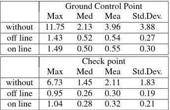
Table 2 presents a comparison between the results obtained with no calibration (CAD design) and each of the two methods. First it is obvious that a photogrammetric-based calibration is necessary to obtain a very good precision on the image models and low image measurement residues. The two photogrammetric methods provide pretty similar results. The residues on check points (0.2) are obviously higher than GCPs because GCPs are compensated whereas check points are not.
Ground Control Point Max Med Mea Std.Dev. without 11.75 2.13 3.96 3.88
off line 1.43 0.52 0.54 0.27 on line 1.49 0.50 0.55 0.30
Check point
Max Med Mea Std.Dev. without 6.73 1.45 2.11 1.83
off line 0.95 0.26 0.30 0.19 on line 1.04 0.28 0.32 0.21
Table 2: Residual on images measurements on ground control points and on check point (in pix.). Max (maximum), Med (Me-dian), Mea (mean), Std.Dev(Standart Deviation)
Ground Control Point Max Med Mea Std.Dev. without 0.125 0.020 0.030 0.029 off line 0.012 0.004 0.005 0.003 on line 0.013 0.004 0.005 0.004
Check point
Max Med Mea Std.Dev. without 1.034 0.269 0.396 0.350 off line 0.092 0.040 0.044 0.023 on line 0.032 0.025 0.023 0.009
Table 3: Residual on ground control points and on check point (in meters). Max (maximum), Med (Median), Mea (mean), Std.Dev(Standart Deviation)
Type of calibration Repartition of image observations in each camera
21 22 23 31 32
Target Network
.
On Line
.
Table 4: Accumulation of image measurement on images plan. im. mes. (image measurments).
off-line and on-line calibration but on CPs, the on-line calibration is better which means that
Another interesting result concerns the distribution of measure-ments in image space. Table 4 shows the difference of density be-tween two methods. The on-line method provides a much higher density and a better sampling of image space due to the accumu-lation of tie points coming from random lanscape contents.
5.2 Pros and Cons
Off-line calibration requires an topometric calibration facility, which is not so easy to build and to maintain. The calibration facility can also be far away from the survey sites and the off-line calibration can thus be done in conditions very different from that of the surveys (e.g. difference in temperature which can have an impact on the mechanical deformation of the metal body on which all the sensors are attached).
On-line calibration use directly the surveys themselves. Thus on the one hand, the number of tie points is potentially much higher and on the other hand the spatial distribution of tie points sample the image space much more densely. One can see on table 4 the repartition of measurements in the different image planes for both calibrations.
The on-line calibration is very efficient and accurate in urban ar-eas but can be unreliable if the environment is not friendly to extract tie points (e.g. forests, etc.).
6 CONCLUSION AND PERSPECTIVE
This paper has presented two complete methods to calibrate a multi-camera mobile mapping system. Although we have adres-sed the specific application of the calibration of a multi-camera panorama head with very low overlap between neighbouring im-ages, the two methods presented can be used for any type of mo-bile platform and any type of multi-camera configuration. The self-calibration method is very interesting from an operationnal point of view, it is fully automatic, it does not need a topomet-ric network, and it adapts itself to the conditions of each survey (mecanic effect oftemperature, etc.). Future work will consist to improve the quality of the on-line calibration by testing, compar-ing and findcompar-ing optimal geometric configurations to realize the calibration in practice (L-shape, S-shape, loop, etc.) and analyze the evolution of the results with the numbers of images.
REFERENCES
Ellum, C. and El-Sheimy, N., 2002. Land-based mobile mapping systems. Photogrammetric Engineering Remote Sensing 68(1), pp. 13–17.
Hartley, R. and Zisserman, A., 2000. Multiple View Geometry in Computer Vision. Cambridge University Press.
Lowe, D. G., 2004. Distinctive image features from scale-invariant keypoints. International Journal of Computer Vision 60(2), pp. 91–110.
McGlone, J., Mikhail, E., Bethel, J. and Mullen, R., 2004. Man-ual of photogrammetry (5th Edition). American Society for Pho-togrammetry and Remote Sensing.
Petrie, G., 2010. An introduction to the technology mobile map-ping systems. GEOInformatics 13, pp. 32–43.
Scheller, S., Westfeld, P. and Ebersbach, D., 2007. Calibration of a mobile mapping camera system with photogrammetric method. International Archives of Photogrammetry, Remote Sensing and Spatial Information Sciences 36 (Part 5/C55), pp. on CD–rom. Schmid, H., 1959. A general analytical solution to the problem of photogrammetry. Technical Report 1065, Ballistic Research Laboratories, US.
Triggs, B., McLauchlan, P., Hartley, R. and Fitzgibbon, A., 2000. Bundle adjustment - a modern synthesis. In: W. Triggs, A. Zisser-man and R. Szeliski (eds), Vision Algorithms: Theory and Prac-tice, LNCS, Springer Verlag, pp. 298–375.