Full Terms & Conditions of access and use can be found at
http://www.tandfonline.com/action/journalInformation?journalCode=ubes20
Download by: [Universitas Maritim Raja Ali Haji] Date: 11 January 2016, At: 22:06
Journal of Business & Economic Statistics
ISSN: 0735-0015 (Print) 1537-2707 (Online) Journal homepage: http://www.tandfonline.com/loi/ubes20
Search With Dirichlet Priors: Estimation and
Implications for Consumer Demand
Sergei Koulayev
To cite this article: Sergei Koulayev (2013) Search With Dirichlet Priors: Estimation and Implications for Consumer Demand, Journal of Business & Economic Statistics, 31:2, 226-239, DOI: 10.1080/07350015.2013.764696
To link to this article: http://dx.doi.org/10.1080/07350015.2013.764696
Accepted author version posted online: 15 Jan 2013.
Submit your article to this journal
Article views: 227
Search With Dirichlet Priors: Estimation
and Implications for Consumer Demand
Sergei K
OULAYEVKeystone Strategy, LLC, Cambridge, MA 02140 ([email protected])
This article is an empirical application of the search model with an unknown distribution, as introduced by Rothschild in 1974. For searchers who hold Dirichlet priors, we develop a novel characterization of optimal search behavior. Our solution delivers easily computable formulas for the ex-ante purchase probabilities as outcomes of search, as required by discrete-choice-based estimation. Using our method, we investigate the consequences of consumer learning on the properties of search-generated demand. Holding search costs constant, the search model from a known distribution predicts larger price elasticities, mainly for the lower-priced products. We estimate a search model with Dirichlet priors, on a dataset of prices and market shares of S&P 500 mutual funds. We find that the assumption of no uncertainty in consumer priors leads to substantial biases in search cost estimates.
KEY WORDS: Consumer learning; Consumer search; Discrete choice models of demand.
1. INTRODUCTION
One of the insights of the theoretical literature on consumer search is the distinction between two types of uncertainty that a searcher may face. One is the uncertainty about current prices, or locations, which makes search necessary. Another is the uncer-tainty about the underlying process that generates these prices. According to Stigler (1961) and McCall (1970), when a con-sumer knows the price distribution, she stops searching as soon as she finds a price below her reservation price. As pointed out by various authors, this stopping rule leads to a search behav-ior with some unrealistic properties. For one, consumers who know the price distribution are perpetually optimistic: they keep searching regardless that they are finding prices that are higher than the reservation price. Another is the no-return property: the consumer always buys from the seller visited last. As shown by de los Santos, Hortacsu, and Wildenbeest (2012a), there are plenty of return patterns in the real-world search data. Finally, one cannot expect consumers to know factors that determine the distribution of prices. Rothschild (1974) was the first to study optimal search under both types of uncertainty. In his model, a searcher holds Dirichlet priors about unknown price distribu-tion, and updates them in a Bayesian way as new price quotes arrive. Instead of a single reservation price, a search is governed by a sequence of increasing reservation prices, as if consumers become less demanding with time.
This article is the first to bring the search model with Dirichlet priors to empirical work. Existing studies of consumer search have relied almost exclusively on the search model from a known distribution: for example, Hong and Shum (2006) and Moraga-Gonzalez, Sandor, and Wildenbeest (2009). The underlying as-sumption has been that a search model where beliefs have zero prior uncertainty delivers a reasonably good approximation of search behavior. We are interested in the implications of devia-tions from this assumption for estimates of search costs and for price sensitivity of the search-generated demand.
Within the framework of search with Dirichlet priors, we develop a novel characterization of optimal search that leads to closed form, easily computable probabilities of purchase of
individual products. This allows us to recover search costs using either individual purchase data or aggregate market shares. As such, it is a useful input for any market-level analysis where consumers search before they buy: studying a firm’s pricing decisions, investment in new products, advertising, and so on.
In the search context, the main difficulty in computing pur-chase probabilities is integrating out unobserved search histories or sequences of price quotes received by the searcher. We show that a direct approach to integration, based on the reservation price characterization, suffers from the curse of dimensional-ity: the cost of numerical integration quickly increases with the number of products. Our approach is based on an observation that a full search history contains more information than what is necessary to compute the probability of purchase. In fact, with Dirichlet priors, only two pieces of information characterize a search: the identity of the second-best product among the dis-covered set, and the length of search preceding the discovery of the best product. All potential search histories are classified by these two variables, breaking down the curse of dimensionality. Using our theoretical results, we show that besides being more realistic the learning process changes consumers’ price responses in a qualitative way. When consumers search, they buy a product in one of two ways: either right away (“fresh demand”), or by returning at a later stage (“returning demand”). In a search with a known distribution, all demand is “fresh”: consumers buy the product either right away, or never. Higher price reduces demand by motivating some of these consumers to continue searching, to never return. In the model with learning, a substantial part of demand is “returning.” Such buyers are neces-sarily more pessimistic than the “fresh” ones: they buy because they failed to find a better deal. Since these searchers find po-tential improvements unlikely, their expected benefit of search is also less sensitive to price increases. As a result, the learn-ing mechanism leads to a less price-sensitive demand overall.
© 2013American Statistical Association Journal of Business & Economic Statistics April 2013, Vol. 31, No. 2 DOI:10.1080/07350015.2013.764696
226
Although it is difficult to generalize this argument for an arbi-trary search cost distribution, this intuition does help explain some of our empirical findings.
We then investigate the empirical relevance of consumer learning. First, we conduct a number of Monte Carlo exercises. In these experiments, we recover parameters of search cost dis-tribution by fitting a search model from a known disdis-tribution on a simulated dataset of prices and market shares generated by consumers who learn while searching. We find that the model without learning consistently overestimates the median search cost. The possible explanation is that since the model without learning delivers more elastic demand, the optimization rou-tine attempts to compensate for it by choosing higher values of search costs to explain the observed price–quantity relationship. The bias increases quickly with variance of the consumer prior: that is, even a small deviation from the assumption of known distribution is consequential.
Next, we apply our model to a real-world dataset of prices (management fees) and market shares of S&P 500 mutual funds, from 1995 to 2000. These data were previously used by Hortacsu and Syverson (2004) to recover search costs from a search model with a known distribution. The results are generally similar to our findings in Monte Carlo experiments: holding the mean prior constant, a moderate degree of prior uncertainty results in substantial biases in estimates of search cost parameters and, consequently, the price elasticity of demand for funds. Similar to Monte Carlo results, the search model with a known distribution overestimates the median search cost, but underestimates the variance. The bias in price elasticity can be either positive or negative, depending on product rank.
Although we believe that the model with learning is more realistic, using data on prices and market shares only is not sufficient to distinguish between the two approaches to search. Specifically, we find that the level of fit is essentially the same for different values of prior variance. The explanation is that a sufficiently flexible specification of search costs is capable of explaining the market shares data, without the need for ad-ditional degrees of freedom coming from unknown priors. To detect learning requires more detailed search data, as we discuss in the concluding section of this article.
In the existing literature, the first derivation of ex-ante distri-butions of outcomes of search, when consumers are learning, is due to Morgan (1985). Building on Kohn and Shavell (1974), Morgan proposed a method to compute reservation values prior to search and used them to find distributions of the length of search and of the final purchase. Unfortunately, his method is computationally intensive, as it involves solving a number of dy-namic problems. Also, the applicable class of beliefs does not include the Dirichlet distribution. Bikhchandani and Sharma (1996) demonstrated that for Dirichlet priors the reservation prices can also be computed prior to search and they conjec-tured that it should be possible to compute ex-ante distributions of search outcomes but did not derive probabilities of purchase. In a related article, de los Santos, Hortacsu, and Wildenbeest (2012b) also considered search with Dirichlet priors and de-veloped a method of recovering search costs through inequal-ity conditions implied by the observed search decisions. Their method requires data on price histories observed by searchers, while ours relies only on market share data.
The literature has also explored other forms of consumer learning, often within the search context. Hendricks, Sorensen, and Wiseman (2012) developed a model of herd behavior, where consumers learn from experience of others, and examined in-efficiencies resulting from the herd behavior. In contrast, in our model, consumers learn only from their own experience. Ackerberg (2003) examined consumer learning in the context of search for experience goods, when consumers are aware of the set of brands (varieties), but have incomplete information about their quality. Crawford and Shum (2005) modeled doc-tors’ learning about the effectiveness of a new drug through experimentation. A more recent article in the healthcare context is Chernew, Gowrisankaran, and Scanlon (2008). Similar to our study, they employed Beta priors (a special case of Dirichlet distribution for two points of support) to model the evolution of consumer beliefs. In their model, consumers received additional signals about the quality of a health plan, which were shown to have substantial impact on health plan choices.
2. THE SEARCH MODEL
2.1 Basic Setup
The following model was originally formulated by Rothschild (1974). A consumer is looking to buy a certain product. Suppose at the time of searchNvarieties are available on the market:
SN = {u1, u2, . . . , uN},
where utilities are sorted in decreasing order, that is,u1 is the
first-best,u2is the second-best, and so on. Therefore, the utility
indexr=1. . . N also stands for the rank of the product. For clarity, we assume that all varieties have distinct utilities (a solu-tion for the case of duplicate utilities is available upon request). As the analysis will proceed from the point of view of a single consumer, we suppress any consumer-specific indices until they become relevant.
A consumer who wishes to make a purchase in this market faces two types of uncertainty. First, she does not know the locations of varieties, which necessitates search. She collects information through a sequence of costly search attempts. The search technology returns a particular ur ∈S with probability
ρr, independently from previous draws. The second type of
uncertainty is that the consumer does not know the actual sam-pling probabilities. Instead, she believes that any search attempt would reveal a utility that belongs to a set of potential utility levels:
SN ⊆SG= {u˜1,u˜2, . . . ,u˜G}.
In the original article, Rothschild (1974) assumed SN =SG,
which corresponds to the case when the consumer knows the set of actual utilities but does not know their locations. Our formulation is more general as it allows for uncertainty about the support of the distribution. In other words, a consumer does not know the probability of sampling a particular price level, including whether this probability is positive.
Because prices are discrete, the assumptionSN ⊆SGfits
nat-urally the context of search for best price; however, it is restric-tive for the general case of continuously distributed utilities. In
that case, we essentially assume that consumers are indifferent between products that have sufficiently similar utilities.
The actual probability pg of sampling ˜ug ∈SG is
deter-mined by the search technology and the availability of products:
pg =ρr(g), ur(g)∈SN, and pg =0 for ur(g) ∈/SN. The
con-The mean prior belief is
E(p1, . . . ,pG)=
The parameter N0 is inversely related to the diffusion of the
prior: the larger it is, the lower is the informational content of new observations. The ratiosαg/N0 represent relative
like-lihoods of elements of SG. As more utilities are sampled,
the consumer updates her beliefs in a Bayesian fashion. Let
Nt =(nt1, . . . , ntG) represent the number of times each utility level has been sampled during search. Standard results imply (see, e.g., Rothschild1974) that the posterior distribution is also Dirichlet, with posterior mean:
According to this updating rule, the relative likelihood of ob-serving a utility levelug ∈SGincreases every time it is sampled.
As the searcher’s information set grows, the posterior mean be-lief converges to the actual sampling technology:E(pg)→ρg
forug∈SNandE(pg)→0 forug ∈/SN.
For all their advantages—flexibility, simplicity, and conjugacy—Dirichlet priors also have a well-known drawback: the updating is local. Sampling a certain utility level affects be-liefs about higher utilities in a uniform fashion, without changing their relative likelihoods. In a more realistic setup, one would expect that sampling some utility level will also raise the rel-ative weight of its neighbors. For example, a prior based on a mixture of normal distributions has this property. However, the normal prior has strong restrictions on the shape of its tails, while Dirichlet distribution has no such restrictions.
2.2 The Optimal Search Decision
A rational consumer continues searching as long as the ex-pected benefit of a search attempt remains above the search cost. Aftertsearches are made, the search history is a sequence of utility levels drawn at every step:ht = {u1, u2, . . . , ut}. Al-ternatively, it can be written as a sequence of indices of ele-ments ofSN that have been sampled:ht = {r1, r2, . . . , rt}. We
adopt the latter representation. SinceSN is ordered, we can
de-finer∗(h)=min{r1, r2, . . . , rt}—the index of the best product found during search.
As shown by Rothschild (1974), a consumer with Dirichlet priors will continue searching aftertattempts if and only if the
following inequality holds (wherecstands for search cost):
Emax(u, ur∗)−ur∗ =
˜
ug>ur∗
( ˜ug−ur∗)E[pg|Nt]> c. (3)
With updating rule (2), the left side of the inequality decreases witht, so the search process is finite. Once the inequality is reversed, the consumer stops and buys the best product out of those discovered during search. As search results are random, the identity of the purchased product is also random. Our goal is to derive the ex-ante (prior to search) probabilities of purchase for a given product, conditional on preferences and search cost. It is notable that not a single sequence of utility draws can arise as a search history. This is because condition (3) must be satisfied recursively, that is, the consumer must optimally decide to continue searching at every step except the last one. To em-phasize this property, we introduce the definition of “feasible” search histories:
Definition 1. A search historyht = {r1, r2, . . . , rt}is
feasi-ble if it is optimal to continue searching after every subhistory,
hl= {r1, . . . , rl},l < t.
LetHrdenote the set of feasible search histories after which
the consumer optimally decides to stop and buyur ∈SN.
The-oretically, the ex-ante purchase probability of productrcan be obtained by summing up probabilities of all histories inHr:
Pr =
h∈Hr
P(h). (4)
2.3 Calculation of Purchase Probabilities by Direct Integration
When the number of products is small, the formula (4) can be computed directly. However, as the number of products in-creases, calculations quickly become unfeasible. Indeed, the summation in Equation (4) is subject to a curse of dimension-ality. For a given search costc, letT(c) be the maximal search length (as shown by Rothschild1974, it is finite, but unbounded as search cost reduces to zero). Because the search is with re-placement, the number of potential search histories is in the order of NT, where N is the number of products. As a re-sult, the computational time involved in summation (4) grows exponentially.
We attempt to compute Equation (4) forT =10 and N =
2,3, . . . ,10. The set of product utilities and their sampling probabilities was taken from the actual data used in our em-pirical application. We construct anNT ×T matrix of all
pos-sible search histories, and for every one we recursively apply formula (3) to determine the optimal stopping decision, and the purchased product. Computations are conducted in Matlab, on a powerful computer cluster, vectorized for speed whenever pos-sible. WithT =10 andN =8, it takes 10 min to evaluate the summation, 30 min forN =9, and 10 hr forN =12. In our empirical application, we have 24 products per market: by ex-trapolation, we find it would take more than a year to compute a purchase probability once.
Another issue with direct application of Equation (4) is that it requires numerical integration over the unobserved search cost.
With 100 draws from the underlying distribution, it will take 10∗100=1000 min for a single evaluation of the objective function, in the case whereT =10 andN =8 . In contrast, the method we develop next allows for analytical integration over search cost, which is both faster and more precise.
2.4 New Characterization of Search
Our approach to this problem is to partition the setHr into
a number of categories, whose probabilities are still simple to compute. We achieve this by removing information about search histories that is not necessary for computing the probability of purchase. Indeed, consider the expected benefit of search after a history with lengthtand with the best productr∗. Using (2),
In the previous formula, we used the fact that since utilities ˜
ug > ur∗ are not sampled, the correspondingntg are all zeros.
Equating the expected benefit to search cost, we obtain the indifference condition
Solving fortand taking into account integer constraints,
¯
Lemma 1. The continuation decision of a consumer with Dirichlet priors after a search historyht depends on two pa-rameters:tis the length of the search history, andr∗is the index of the best utility sampled during search. Given these parame-ters, the consumer continues searching if and only if
t <k¯r∗. (8)
Proof. Consider Equation (6). The left side—the expected benefit of search aftertattempts—is decreasing int. Ift >k¯r∗,
the benefit of search falls below search cost, and the search stops. The same is true fort =k¯r∗, because ¯kr∗ is obtained by
upward rounding of the solution to Equation (6).
Therefore, the length of the search historyt and the index of the best productr∗ are sufficient to determine the optimal continuation decision. According to Lemma 1, when a searcher with Dirichlet priors finds a better product, in her continua-tion decisions she “forgets” the previously found products and “remembers” only the length of prior search.
Computing Equation (7) for r=1, . . . , N, we obtain the vector of sufficient statistics that completely summarizes search behavior:
¯
k= {k¯1,k¯2, . . . ,k¯N}. (9)
The advantage of this characterization is that the length of the ¯
k vector is fixed, as opposed to the sequence of reservation utilities, whose length is unbounded. A further observation from Equation (7) follows:
Lemma 2. A consumer with Dirichlet priors will search longer if inferior products are sampled. Formally, let h1 and h2be two histories of the same length, buth1 has inferior best
product than h2: r∗ > r∗∗. Then, if the consumer decides to
continue searching afterh2, then he necessarily continues after h1, too.
Proof. According to Equation (8), the consumer continues afterh2ifft <k¯r∗. From Equation (7), ¯kr is decreasing inur,
or, alternatively, increasing inr. Therefore, ¯kr∗∗≥k¯r∗> t and
the search continues afterh1as well.
During a search with an unknown distribution, sampling a low-utility product has two opposite effects on the incentives to search: it makes sampling higher utilities less probable, discour-aging search; and it decreases the status quo, promising larger potential improvements. As Lemma 2 finds, a consumer will search longer if inferior products are sampled; therefore, the second effect dominates.
2.5 Probability of Purchase
Reversing condition (8), we can see that all histories leading to a purchase of productr∗must satisfyt ≥k¯
r∗. However, not
all sequences of utility draws that correspond to the same pair (t, r∗) are feasible. Additional information about a search history is necessary to determine its feasibility.
Lemma 3. A search historyht= {r1, r2, . . . , rt}is feasible
if and only if it is optimal to continue searching after the penul-timate subhistory,ht−1 = {r1, r2, . . . , rt−1}.
Proof. Denote by r∗
t−1 the best product found during ht−1.
Assume first that it is optimal to continue searching afterht−1
. Lemma 1 implies that t−1<k¯r∗
t−1. Consider any subhistory hl= {r1, . . . , rl},l < t−1. Since longer search can only
im-l (see Lemma 2). Therefore, it is optimal to
con-tinue searching afterhl:l < t−1<k¯r∗
t−1≤k¯rl∗. The converse
is true, because if a historyhtis feasible, then by definition it is
optimal to continue searching after every subhistory, including
ht−1.
It follows that, in addition to the search length and the index of the best product, we need to knowr∗
t−1, which is the index of
the product that prevailed on the penultimate subhistory,ht−1.
Together, inequalitiest >k¯r∗ andt−1<k¯r∗
t−1 ensure that the
feasibility of a search history leads to a purchase of productr∗. Further, observe that any search history leading to product
r∗ can be divided into three stages. First, there is an initial stage where inferior products are sampled. Denote by t0 the
length of that stage, and by r∗∗ the index of the best product found during that stage, which is also the second-best for the entire search history. Then, the product r∗ is sampled at the periodt0+1. Finally, during the third stage, products indexed r≥r∗are sampled until the search is stopped. If the first stage is empty, that is, the search started by sampling the best product, we
haver∗
t−1=r∗; if not, thenrt∗−1=r∗∗. Therefore, the feasibility
of a search history can alternatively be stated as a condition on the second-best product. This intuition is formalized in the following proposition.
Proposition 1. For a consumer with Dirichlet priors, a search historyht = {r1, r2, . . . , rt}is feasible and results in a purchase of productr∗if and only if it satisfies the following conditions:
r∗=min{r1, r2, . . . , rt}
t0<k¯r∗∗ (10)
t =max{t0+1,k¯r∗},
wheret0is the length of the search history beforer∗is
discov-ered;r∗∗ is the index of the second-best product; andtis the length of the search history.
Proof. Together with r=r∗, the condition t =max{t
0+
1,k¯r}impliest ≥k¯r∗, which is a necessary and sufficient
condi-tion for optimal stopping, by Lemma 1. Therefore, we only need to establish feasibility. Assume first that for a historyhtthe
sys-tem (10) is satisfied. Suppose thent =t0+1, that is, the search
stopped as soon as the productrwas sampled (so the third stage is empty). Inequalityt0 <k¯r∗∗implies that, according to Lemma
1, it is optimal to continue after the penultimate subhistory,
ht0 =ht−1. By Lemma 3,ht is feasible. Suppose alternatively
thatt =k¯r > t0+1. Sincer=r∗andt−1<k¯r, such a
his-tory is feasible too. Conversely, assume that a hishis-tory is feasible. The conditiont0<k¯r∗∗holds because by definition it is optimal
to continue searching under every subhistory, includingt0. If t0+1<k¯r, the search continues untilt =k¯r; if t0+1≥k¯r,
the search optimally stops as soon as product r is sampled; generalizing both cases, we obtaint =max{t0+1,k¯r}.
Following this result, all variety of histories that belong to
Hrcan be divided into exactly ¯kNclasses, indexed by length of
the first stage, t0=0,1, . . . ,k¯N−1. The identities of goods
that are sampled during that stage do not matter, as long as only products inferior tor∗ are sampled and the search optimally continues after that. The probability measure of Hr becomes
straightforward to compute.
Proposition 2. In a search process with Dirichlet priors, the ex-ante probability of purchasing a good rankedr =r∗is found as
Proof. It follows from Proposition 1 that the union of all t0
classes is equal toHr. Givent0, the set of products sampled
dur-inght0must satisfy two criteria: they must be inferior to product v; the best among them,r∗∗, must satisfyt0 <k¯r∗∗. Since ¯kr is
nondecreasing inr, the latter inequality impliest0<k¯rfor any
r≥r∗∗. Combining these conditions, we obtain that products
r≥r¯(r∗, t
0) can be sampled during the first stage. The
probabil-ity of this happening exactlyt0times is (ρr¯(r,t0)+ · · · +ρN)
t0. On
the second stage, goodr∗is sampled with probabilityρ
r∗. After
that, the searcher must continue sampling goodsr∗, . . . , N ex-actly max(0,k¯r∗−t0−1) times. A special provision is needed
for the case ofr∗=N, because the first stage is empty. So far, we have assumed that all utilities inSN are distinct.
A result analogous to Equation (11) for the case of duplicate utilities is available from the author upon request.
2.6 Rationality of Beliefs
In the search model from known distribution, rationality of beliefs typically amounts to an assumption that consumers know the empirical distribution of utilities. In the model with learning, the implications of the rationality requirement are less clear. Here, we will assume that while consumers are uncertain about the actual sampling probabilities, their mean prior is correct:
E[pg]=ρg, if ug ∈SN
=0, if ug ∈/SN. (12)
In particular, the rationality requirement implies that the set of potential utilities,SG, coincides with the set of actual ones,
SN, which is a restrictive assumption, as we argued previously.
In our empirical application, we will additionally compute a specification where this assumption is relaxed. Conceptually, the caseSG=SNonly affects the values of sufficient statistics,
¯
k1,k¯2, . . . ,k¯N(see Equation (7)). Conditional on this vector, the
optimal stopping decisions and probabilities depend only on the set of actual utilities,SN. By introducing nonexistent utilities
into the consumer prior, we effectively increase the variety of potential search results, thus inducing consumers to search more than they would otherwise.
3. MARKET SHARES
3.1 Model With Learning
The market share of an individual product will be an aggregate result of searches performed by many consumers. These con-sumers are endowed with a search cost as a draw from the pop-ulation level CDF of search cost distribution:ci ∼F(c). In
ad-dition, utilities of available products,SN = {u1i, u2i, . . . , uN i},
may differ across consumers. The market share of a product
j—a purchase probability by a random consumer—is computed by integrating out these unobservables:
Qj =
purchasing productjby consumeriwhere the product’s rank is
r. This expression was derived in Equation (11).
In applications, we assume search for the best price, that is,
uj = −pj. In this case, the ranking of utilities is observable
(e.g., j =r), and consumers differ only by search cost. The
market share function becomes
In the second equation, the functions ¯kj(c, pj) are integer-valued
and decreasing in the search cost. Therefore, there is a set of search cost intervals such that the entire vector ¯k2, . . . ,k¯N is
constant within each interval. Since the purchase probability
Pr depends only on this vector, it is also constant within such
intervals. We use this insight to integrate out unobserved search costs analytically.
Define a matrix of search cost cutoffs:
¯
support for search costsc∈(0,+∞) guarantees the existence. Although ¯ki can be arbitrarily large for small-enough values
of search cost, in practice, an upper bound ¯ki< Kwill give an
adequate approximation. (Implicitly, this defines a small interval of search costs, [0, cmin(K)], over which we assume a constant
probability of purchase)
Sorting the set of cutoffs{c¯kr}in an increasing order, we ob-tain a set of intervals [ ˜cs,c˜s+1),s=1, . . . , Ns, such that the
probability of purchase is constant within each. Specifically, for anyc∈[ ˜cs,c˜s+1), we have ¯kr(c, pr)=k¯rs,r=2, . . . , N, which
implies a purchase probabilityPrs =Pr(1,k¯2s, . . . ,k¯
s
N).
Return-ing to Equation (14), we obtain the market share of productr
as:
In the search model with a known distribution, the predicted market shares are straightforward to compute. Letρg be the
probability of finding productgon the next search attempt. In terms of our learning model, ρg =αg/N0. Given a vector of
prices, define search cost cutoffs as
¯
cr =
g<r
ρr(pr−pg), r=2, . . . , N. (17)
Consumers withc >c¯rwill stop searching and buy goodrupon
sampling it, while others will continue searching. The set of po-tential buyers for productrconsists of a sequence of intervals: [ ¯cr; ¯cr+1),[ ¯cr+1; ¯cr+2), . . . ,[ ¯cN,+∞). In the first interval,
con-sumers will stop searching as soon as they find any price lower
or equal to pr, which implies the probability of buying good
rasρr/(ρ1+ · · · +ρr). For search costs from [ ¯cr+1; ¯cr+2), the
potential set of purchases includesp1, . . . , pr+1, so the
proba-bility of buyingrisρr/(ρ1+ · · · +ρr+1). The predicted market
share of goodris the sum of demand by consumers from each interval, weighted by their population shares:
Qr(p1, . . . , pN)=
A simple example helps illustrate the application of formulas for market shares. Suppose only three prices are available:p1=
0, p2 =1, p3 =2. Beliefs are represented by a uniform prior: α1=α2=α3=1,N0=3. Accordingly, the actual sampling
technology is uniform, with replacement. Applying formula (7),
¯
we obtain sufficient statistics for search with learning: ¯k2(c)=
max(1,ceil(1cp2−3))=max(1,ceil(1c−3)), k¯3(c)=max(1,
ceil(1c(2p3−p2)−3))=max(1,ceil(31c−3)). For the highest
ranked product 1, ¯k1(c)≡1. Solving equations ¯k2 =1,2, . . . ,5
and ¯k3=1,2, . . . ,6, we obtain a set of search cost cutoffs.
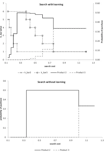
These cutoffs divide the search cost line in a number of inter-vals, as shown on the x-axis of Figure (1), upper panel. For search cost values within an interval, both statistics ¯k2(c),k¯3(c)
are constant (see lines “kbar2” and “kbar3” in the figure). Be-cause the probabilities of purchase of products 2 and 3 are completely determined by these statistics, they are also constant within an interval. In this case, the formula (11) reduces down to:
In the model without learning, there is only one cutoff per product: ¯c2=13p2 and ¯c3= 13(2p3−p2). Observe that these
cutoffs are close to ¯c21and ¯c13in the learning model, respectively. Forc∈[ ¯c2,c¯3), product 2 is bought with probability 1/2, and
for c≥c¯3 with probability 1/3. For low search costs, c <c¯3,
product 3 is not bought: consumers who find it continue search-ing. In contrast, in the learning model, any product has a positive chance of being bought: even a consumer with low search cost may have a sufficiently unlucky search experience that would prompt her to stop and return to the product.
0.00 0.10 0.20 0.30 0.40 0.50 0.60
0 1 2 3 4 5 6 7
0.1 0.3 0.5 0.7 0.9 1.1 1.3
Probability of
purchase
k_bar value
search cost
Search with learning
k_bar2 k_bar3 Product 2 Product 3
0 0.1 0.2 0.3 0.4 0.5 0.6
0.1 0.3 0.5 0.7 0.9 1.1 1.3
probability of purchase
search cost
Search without learning
Product 2 Product 3
Figure 1. Probability of purchase as a function of search cost, for models with and without learning. The upper panel also displays values of ¯k2
and ¯k3as a function of search cost. Notice the correspondence between changes in the values of ¯k2and ¯k3and changes in purchase probabilities.
4. LEARNING AND PRICE ELASTICITY
When consumers learn while searching, the optimal stopping rule of Proposition 1 determines whether a consumer who just found a product will buy it now or will return to it in the future. How does the likelihood of these events change if the seller increases the price by a certain amount? How does the learning process shape the consumer’s price response?
For both types of search models, define the price elasticity of demand for productras the normalized derivative of its market share:
ǫr =
∂Qr(p1, ., pr, ., pN)
∂pr
pr
Qr
. (20)
We compare this quantity between models with and without learning, using results derived in the previous section.
When applied to search-generated demand, the notion of price elasticity can take two different meanings. A “short-term” price elasticity refers to price changes that are sufficiently recent so that they are not yet incorporated in prior beliefs. Consequently, the short-term change in demand comes only from search de-cisions made by consumers who discovere the new price. A “long-term” price elasticity refers to a demand response where the new price is already incorporated in prior beliefs. In this case, a price change affects search behavior of all consumers. This implies a higher competition from rival products, as more con-sumers who discover a rival product now stop and buy instead of continuing to search.
Search cost Cutoffs for
good 3
Cutoffs for good 2 Demand for good 2
P(1,2,12)
0 P(1,2,9)
P(1,2,2)
1/3 Search with learning
Search cost Cutoffs for
good 3
Cutoffs for good 2 Demand for good 2
0 1/2
1/3 Search without learning
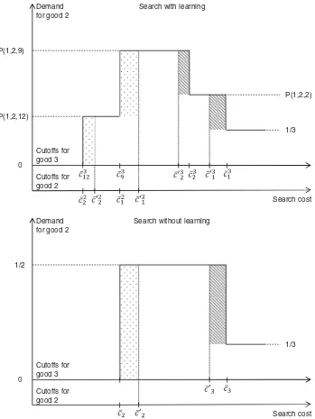
Figure 2. Comparing price responses in search models with and without learning. Dotted areas are short-term losses in demand for product 2, while long-term losses are a sum of both dotted and dashed areas.
To see the implications of the learning process for both short-and long-term price elasticities, it is useful to distinguish be-tween two components of demand for a search product. The “fresh” demand comes from consumers who bought the prod-uct immediately upon discovering it. The “returning” demand is from those who found the product and continued searching, but unsuccessfully: failing to find a better deal, they returned and made the purchase.
In search without learning, all demand is “fresh”: searchers either buy the product right away, or never. In the three-product example, only consumers withc >c¯2buy product 2,
immedi-ately upon discovery. FromFigure 1, lower panel, we can see that demand for product 2 also depends on the cutoff for product 3, ¯c3. Following a short-term price increase for product 2, its
cutoff increases, ¯c′
2>c¯2, while ¯c3 is not affected. In the long
run, the same price change also decreases product 3’s cutoff: ¯
c3′ <c¯3. Therefore, in the short run new cutoffs are ¯c′2,c¯3 and
in the long run, ¯c′
2,c¯
′
3.Figure 2, lower panel, depicts the
corre-sponding changes in demand for product 2. The dotted area is a short-run loss in demand, from consumers who sampled prod-uct 2 but continued searching. The long-run change additionally includes the dashed area, from consumers who sampled product 3 before discovering product 2.
With learning, the behavior of consumers with a search cost
cis described by a set of sufficient statistics, ¯k1(c), . . . ,k¯N(c),
where ¯k1≡1 as a normalization. Define a set of search cost
cutoffs for products 2 and 3:
¯
ck2= 1
k+3α1(p2−p1), k=1, . . . ,2 (21) ¯
ck3= 1
k+3(α2(p3−p2)+α1(p3−p1)), k=1, . . . ,12. (22)
Figure 2, upper panel, depicts demand for product 2. There are two horizontal axes, one for product 2’s cutoffs and another for product 3’s. Previously, Figure 1, upper panel, combined both sets of cutoffs on a single line. “Fresh” demand for product 2 comes from consumers withc >c¯21, while “returning” con-sumers are between ( ¯c22,c¯21) (to save space, we omit the part of demand curve for smaller costs). Similar to the model without learning, a short-term price change only increases product 2’s own cutoffs, ¯ck′2>c¯2k; a long-run change will decrease all of its rival’s cutoffs: ¯c′k3<c¯3k.
Comparing upper and lower panels, we observe that the sum of short-term losses in the model with learning is smaller than in the model without learning. That is, the short-term price elastic-ity is smaller if consumers learn while searching. The reason is that consumers from various intervals of search costs will react differently depending on whether or not they are learning.
Consider first consumers who belong to the interval ( ¯c2
1,c¯′12).
Before the price change, they were part of “fresh” demand, buying the product with probabilityP(1,2,9). After the price change, they become “returning,” who are less likely to buy the product:P(1,2,12)< P(1,2,9). Further, consumers from ( ¯c22,c¯′22) were initially part of the “returning” group, but stopped buying the product altogether after the price change. In sum, a short-term price increase leads to a redistribution of demand from “fresh” to “returning,” and from “returning” to zero. The key observation is that the interval ( ¯c2
2,c¯
1), as more consumers enter “returning” demand than drop
out. As a result, the relative change in total demand is smaller than in the model without learning, where all consumers who quit the “fresh” category stop buying the product. The underly-ing reason is given in Remark 1.
Remark 1. In a search with Dirichlet priors, more pessimistic consumers are less sensitive to price changes.
Suppose a consumer has madensearch attempts, where prod-uct 2 was sampled at least once, while prodprod-uct 1 was never sam-pled. From Equation (5), the expected benefit of future search is
EU2= n+13(p2−p1). It increases withp2, but at a smaller rate
with largern. Indeed, if improvements are unlikely, the expected benefit is less sensitive to changes in status quo. Since consumers from the interval ( ¯c22,c¯21) only buy product 2 aftern=2 search attempts, they are more pessimistic than consumers withc >c¯21 who buy product 2 immediately.
To summarize, the learning process makes demand less elastic for two related reasons. First, a portion of demand in the model with learning comes from returning consumers, who are nec-essarily more pessimistic than the “fresh” ones, and hence less price-sensitive. In contrast, consumers who do not learn are per-petually optimistic. Second, the loss in demand from the “fresh” component is partially compensated by an increase in the “re-turning” one, as a result of redistribution of these consumers between two groups. Higher-ranked products have higher share of returning consumers and for them we expect the largest discrepancy between the predictions of two models.
While this simple example is helpful to build intuition, de-veloping a general result is beyond the scope of this article. The gap between price elasticities depends on the shape of search cost distribution, allocation of products, and so on. In the em-pirical application, all these parameters are known (including
the search cost distribution, which is estimated), so the price elasticity comparisons are possible.
5. MONTE CARLO EXPERIMENTS
We conduct a number of Monte Carlo experiments that aim at the following question: What are the consequences of applying a search model from a known distribution to choice data that are generated by searchers who learn? We are particularly interested in how biases in search cost estimates and price elasticities depend on market conditions and belief parameters.
A Monte Carlo experiment is organized as follows. A vector of prices is simulated, one for each market, and there are multiple markets. Under the “true” search cost distribution, log-normal, with parameters E(log(c))= −2.5 and SD(log(c))=0.5, we compute market shares under the assumption that consumers learn while searching (Equation (16)), separately for each
0.00
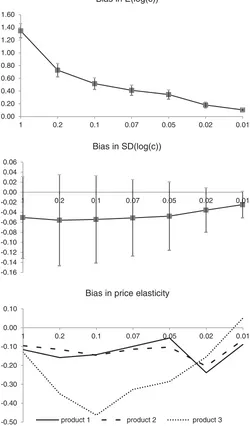
Figure 3. Monte Carlo results. Distribution of biases ( ˆθ−θ), by the variance of the prior. For search cost estimates, 95% confidence intervals are shown.
market. On the simulated data, we estimate a search cost den-sity by fitting the model without learning, with predicted market shares given by Equation (18). Taking the difference between price elasticities obtained under the true model and under the es-timated model, we obtain a measure of a bias. Simulating market share data many times, we obtain a distribution of biases, which is described by the average bias and 95% confidence interval around it.
We repeat the experiment for different values of the variance of prior beliefs, which is a key parameter that differentiates the two models. A smaller variance of the prior brings the model closer to the search without learning, which is a special case with zero variance. The difference between the two models is computed for three parameters: median search cost, variance of search cost, and price elasticity. For reference, the “true” search cost parameters areE(log(c))= −2.5 and SD(log(c))=0.5.
Figure 3presents average biases in these parameters and sim-ulated 95% confidence intervals, by the order of decreasing variance. For example, for variance=1, the bias inE(log(c)) is 1.4, meaning that the model without learning overestimated this parameter by 1.4/2.5=56%. The lower panel represents biases in price elasticities for the top three products. Price elas-ticities are overestimated in all cases, to a varying degree. It is notable that the bias for the third-best product is often much larger, which points to our earlier conclusions about the role of product rank in price elasticity. The size of the bias is not strictly monotonic with the variance of the prior, but generally gets smaller for small values of that parameter. For example,
doubling the variance of the prior from 0.1 to 0.2 increases the bias by 40%.
6. APPLICATION: SEARCHING FOR MUTUAL FUNDS
6.1 Model
Suppose a consumer would like to invest her money into an S&P 500 mutual fund. Since the goal of such funds is to mimic the behavior of the S&P 500 index, their expected returns should be similar. Hortacsu and Syverson (2004) (hereafter, HS) con-firmed this prediction with data on actual returns from mutual funds. They also emphasized a wide variation in management fees across what seem to be similar investment options. One explanation for the observed price dispersion is that investors have nonnegligible search costs and make their investment de-cisions using incomplete information.
Similar to HS, we explore this hypothesis by fitting a search model to the observed relationship between prices and market shares of mutual funds. Our data consist of years from 1995 to 2000, and each year is assumed to represent a separate market. The number of operating funds every year is Nt =24,22,45,57,68,82, which is also the number of
products in the search model. Market shares are formed by search decisions of investors looking for a fund with the lowest management fees. Observed prices are measured in basis points, as a fixed fee per 10,000 dollars invested.Figure 4plots data for 2000.
-14 -12 -10 -8 -6 -4 -2 0
-7 -6.5 -6 -5.5 -5 -4.5 -4 -3.5
log price vs log market share, 2000
log market share
eci
r
p
g
ol
Figure 4. Log-price versus log-market share for funds available in year 2000.
The main point of departure in our approach from HS is that searchers learn from their own experience. In parallel, we estimate a model without learning (following a specification similar to the one found in HS), and compare the outcomes of both models. This allows us to examine the consequences of ignoring consumer learning during the search process: resulting biases in search costs and price elasticity.
We assume search for best price, abstracting away from other sources of fund-level heterogeneity. Suppose prices are sorted in an increasing order, so that indexjalso stands for the ranking of fundjin the set of utilities:p1<· · ·< pNt, whereNt is the
total number of funds in yeart. Every investor is endowed with an idiosyncratic search cost, an iid drawn from a log-normal distribution:
ln(ci)∼N(µ0+µ1t, δ0+δ1t).
For flexibility, both the mean and the standard deviation of search costs contain a time trend. Parametersµ0, µ1, δ0, δ1 are
to be estimated. The search technology is such that fund jin yeartis sampled with a probability:
ρj t =
jin yeart. Parameterγ will be estimated together with search cost parameters. Aγ >0 would indicate that older funds have better exposure, that is, higher probability of being considered by searchers.
In the search model from known distribution, searchers are assumed to know the sampling probabilities (Equation (23)) as well as their support: the vector of available prices,P1, . . . , PN t
in the yeart. However, they do not know what fund offers what price, hence the need for search.
In the model with learning, we relax the assumption that searchers know the distribution of prices. To be sure, data on prices and market shares are not sufficient to identify what their actual priors could be. A sufficiently flexible specification of preferences and search costs is capable of explaining market share data, without the need for additional degrees of freedom coming from unknown priors. We avoid making an arbitrary choice of priors by imposing a rationality requirement, as de-fined in Section (2.6), Equation (12): the mean prior reflects the actual search technology, but searchers are uncertain about it and revise their beliefs while searching. In the adopted notation, we assume thatαj t=ρj tN0,j =1, . . . , Nt. We will additionally
analyze the model where the rationality assumption is relaxed. The parameter N0 is inversely related to the diffusion of
the prior, and we set it N0=Nt in every year, which gives a
relatively small variance. Following the results of Monte Carlo experiments, the bias increases variance of the prior.
Parameters of the search cost distribution are identified from the joint variation of price and market shares, holding the fund’s age constant: the slope of the observed market share function identifies the mean, while the range of observed prices and mar-ket shares identifies the standard deviation of search costs (e.g., substantial variance of search costs is needed to explain cases where a high-priced fund has a significant market share). The pa-rameterγis identified by the joint variation of fund age and
mar-ket shares, holding prices constant, together with an exclusion restriction that the fund’s age does not enter consumer utility.
6.2 Estimation Results
Parameters to be estimated areθ = {µ0, µ1, δ0, δ1, γ}—four
parameters of the search cost distribution, plus the effect of the fund’s age on its sampling probability. The estimation is by nonlinear least squares, where we minimize the weighted sum of deviations between the observed and predicted market shares:
min
Table 1presents estimation results. Column M0 contains es-timates of a model without learning, and column M1 contains estimates from the model with Dirichlet priors. Overall, the level of fit is remarkably good for both models, withR2around 98%. This gives a certain confidence in the empirical relevance of the search model for the best price. While it is plausible that funds may differ in dimensions other than price, the high level of fit
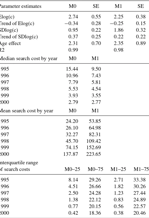
Table 1. Estimates of the distribution of search costs from models of search with (M1) and without (M0) learning. Search costs are expressed in basis points, that is, dollars per 10,000 investment.
Bootstrapped standard errors in the columns are labeled “SE”
Parameter estimates M0 SE M1 SE Elog(c) 2.74 0.55 2.25 0.38 Trend of Elog(c) −0.34 0.28 −0.25 0.15 SDlog(c) 0.95 0.22 1.86 0.32 Trend of SDlog(c) 0.37 0.25 0.22 0.22 Age effect 2.31 0.70 2.35 0.89 R2 0.99 0.98
Median search cost by year M0 M1 1995 15.44 9.50 Mean search cost by year M0 M1 1995 24.20 53.85
of search costs M0–25 M0–75 M1–25 M1–75 1995 8.14 29.26 2.71 33.38 1996 4.51 26.66 1.82 30.26 1997 2.50 24.28 1.23 27.44 1998 1.38 22.12 0.83 24.89 1999 0.77 20.15 0.56 22.57 2000 0.42 18.36 0.38 20.46
-4 -3.5 -3 -2.5 -2 -1.5 -1 -0.5 0
1 2 3 4 5 6 7 8 9 10 11 12 13 14 15
Price elasticities in 1995 (by rank of fund)
M1 M0 M0(M1)
-7 -6 -5 -4 -3 -2 -1 0
1 2 3 4 5 6 7 8 9 10 11 12 13 14 15
Price elasticities in 2000 (by rank of fund)
M1 M0 M0(M1)
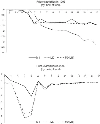
Figure 5. Price elasticities of individual funds, in 1995 and 2000, from models of search with (M1) and without (M0) learning. The line M0(M1) is by M0 with estimates from M1.
in our specification suggests that adding more controls should not change our results qualitatively. Models M0 and M1 give essentially the same level of fit, which reflects the fact that data on market shares do not allow us to detect learning. We have attempted to estimate M1 at different values ofN0, with the
same level of fit.
The median search cost is found to be 9.5 dollars per 10,000 invested in 1995, according to model M1. The model without learning gives a larger estimate, 15.4 dollars. In general, for all years, M0 gives a larger search cost median. This finding is in line with our theoretical and Monte Carlo analysis, which concluded that, holding search cost parameters constant, M0 delivers larger price elasticities than M1. During the estimation, this divergence is in part compensated by choosing a larger search cost median (as consumers with larger search costs are less elastic).
Further, M1 delivers larger standard deviations of search cost for every year; given a log-normal distribution, this results in higher search cost means.
Taken together, the differences in estimates of search cost me-dian and variance have an ambiguous effect on price elasticity. Figure 5compares individual price elasticities as predicted by models M0 (dotted line) and M1 (solid line). For 1995, when the difference in the median estimates was the largest, M0 pre-dicts smaller price elasticities for higher-ranked funds, but the relationship is reversed for the lower-ranked ones.
In principle, both the structure of the model (learning mech-anism) and the difference in search cost estimates could be responsible for the gap in price elasticities. To illustrate the contribution of both factors, the dashed line represents price elasticities computed using M0 with estimates from M1. In this case, we find that biased estimates explain most of the gap, except for the highest-ranked funds. For the latter, the learn-ing mechanism delivers lower price elasticities. For 2000, the search cost medians for M0 and M1 are almost the same, but M1 predicts much higher variance. As a result, we find that M0 sub-stantially overestimates price elasticities for the top five funds in that year, while for lower-ranked funds results are similar. In
-2.5 -2 -1.5 -1 -0.5 0
1 2 3 4 5 6 7 8 9 10 11 12 13 14 15 16 17 18 19 20 21 22 23 24
Price elasticities
original new
0 0.02 0.04 0.06
0.08
0.1 0.12 0.14
1 2 3 4 5 6 7 8 9 10 11 12 13 14 15 16 17 18 19 20 21 22 23 24
fund rank
Predicted market shares
original
new
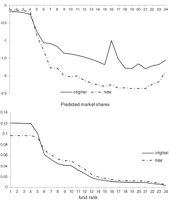
Figure 6. Price elasticities and predicted market shares for individual funds in 1995, before and after adding a grid of nonexistent prices to consumer’s beliefs. Uniform prior assumed in both cases. Estimates of search costs are from M1.
contrast to 1995, this gap is mostly explained by the structure of the model, rather than estimates (see the location of the dashed line).
Figure 6 presents the results of a counterfactual exercise where the assumption of rational beliefs is violated. Specifically, we introduce an equally spaced grid of nonexistent prices, into the prior beliefs held by consumers in 1995. Adding nonexistent utilities in consumers’ beliefs introduces virtual competition to the existing products, motivating consumers to search further. Interestingly, it does so in a way that redistributes market shares from top to lower-ranked products. Due to higher competition, the elasticity of demand for all products increases.
7. CONCLUSIONS
We have studied the behavior of a consumer who is searching for the best product on the market, but who is uncertain about the true distribution of prices. For such a searcher, every search result is a new piece of information about the underlying price distribution, which she uses to update her beliefs in a Bayesian way. For the case of Dirichlet priors, we developed a method
of computing the ex-ante probabilities of purchases, resulting from a search. We used our method to estimate a search model with an unknown distribution, on a dataset of prices and market shares of S&P 500 mutual funds. On the same data, we also estimated a search model from a known distribution, which is a limiting case where the prior uncertainty is set to zero. We found that both models lead to divergent predictions regarding the price elasticity of the search-generated demand. As a result, the assumption of zero prior uncertainty leads to substantial biases in estimates of search costs.
Even though the data on prices and market shares itself does not allow us to test for learning, a conscious choice of a search model should be made in an empirical application. Search from an unknown distribution is a more realistic model: it is difficult to expect consumers to be so confident in their beliefs as to ignore additional information contained in every search result. At the same time, this type of model is thought to be more difficult to estimate, which probably explains its limited use in empirical applications. The method developed in this article significantly reduces this gap, at least if one is willing to accept the assumption of Dirichlet priors.
Several possibilities are left to be explored in future research. The most important one, in our view, is exploring the possi-bilities for identification of the parameters of prior beliefs. In this article, we had to make an assumption about the mean and the variance of the prior, as these parameters were not identified from the market shares only. We conjecture that, to identify these parameters, one must have search data that include search ac-tions as well as observation histories. Variation in characteristics of previously found products will produce variation in posterior beliefs; at the same time, the rationality of the observed search decisions will impose inequality conditions on the parameters of these beliefs.
ACKNOWLEDGMENTS
The author isgrateful to the editor, associate editor, and anony-mous referees whose suggestions have led to substantial im-provements in the article.
[Received September 2011. Revised November 2012.]
REFERENCES
Ackerberg, D. (2003), “Advertising, Learning, and Consumer Choice in Expe-rience Good Markets: A Structural Empirical Examination,”International Economic Review, 44, 1007–1040. [227]
Bikhchandani, S., and Sharma, S. (1996), “Optimal Search With Learning,” Journal of Economic Dynamics and Control, 20, 333–359. [227] Chernew, M., Gowrisankaran, G., and Scanlon, D. (2008), “Learning and the
Value of Information: Evidence From Health Plan Report Cards,”Journal of Econometrics, 144, 156–174. [227]
Crawford, G., and Shum, M. (2005), “Uncertainty and Learning in Pharmaceu-tical Demand,”Econometrica, 73, 1137–1173. [227]
de los Santos, B., Hortacsu, A., and Wildenbeest, M. (2012a), “Testing Models of Consumer Search Using Data on Web Browsing and Purchasing Behavior,” American Economic Review, 102, 2955–2980. [226]
——— (2012b), “Search With Learning,” Working paper, Kelley School of Business, Indiana University. [227]
Hendricks, K., Sorensen, A., and Wiseman, T. (2012), “Observational Learning and Demand for Search Goods,”American Economic Journal: Microeco-nomics, 4, 1–31. [227]
Hong, H., and Shum, M. (2006), “Using Price Distributions to Estimate Search Costs,”RAND Journal of Economics, 37, 257–275. [226]
Hortacsu, A., and Syverson, C. (2004), “Product Differentiation, Search Costs, and Competition in the Mutual Fund Industry: A Case Study of S&P 500 Index Funds,”Quarterly Journal of Economics, 119, 403–456. [227,235] Kohn, M., and Shavell, S. (1974), “The Theory of Search,”Journal of Economic
Theory, 9, 93–123. [227]
McCall, J. (1970), “Economics of Information and Job Search,”Quarterly Jour-nal of Economics, 84, 113–126. [226]
Moraga-Gonzalez, J., Sandor, Z., and Wildenbeest, M. (2009), “Consumer Search and Prices in the Automobile Market,” Working paper, IESE Busi-ness School, University of Navarra. [226]
Morgan, P. (1985), “Distributions of the Duration and Value of Job Search With Learning,”Econometrica, 53, 1199–1232. [227]
Rothschild, M. (1974), “Searching for the Lowest Price When the Distribu-tion of Prices Is Unknown,”Journal of Political Economy, 82, 689–711. [226,227,228]
Stigler, G. J. (1961), “The Economics of Information,” Journal of Political Economy, 69, 213–225. [226]