Modification of DAISY SVAT model for
potential use of remotely sensed data
Peter van der Keur
a,∗, Søren Hansen
a, Kirsten Schelde
b, Anton Thomsen
baDepartment of Agricultural Sciences, The Royal Veterinary and Agricultural University, Laboratory for Agrohydrology and Bioclimatology, Agrovej 10, DK-2630 Taastrup, Denmark
bDepartment of Crop Physiology and Soil Sciences, Danish Institute of Agricultural Sciences, Research Centre Foulum, P.O. Box 50, DK-8830 Tjele, Denmark
Received 30 April 1999; received in revised form 7 August 2000; accepted 19 August 2000
Abstract
The SVAT model DAISY is modified to be able to utilize remote sensing (RS) data in order to improve prediction of evapotranspiration and photosynthesis at plot scale. The link between RS data and the DAISY model is the development of the minimum, unstressed, canopy resistancermin
c during the growing season. Energy balance processes are simulated by
applying resistance networks and a two-source model. Modeled data is validated against measurements performed for a winter wheat plot. Soil water content is measured by time domain reflectometry. Crop dry matter content and leaf area index are modeled adequately. Modeled soil water content, based on a Brooks and Corey [Brooks, R.H., Corey, A.T., 1964. Hydraulic properties of porous media. Hydrology Paper no. 3, Colorado University, Fort Collins, CO, 27 pp.] parameterization, from 0 to 20, 0 to 50 and 0 to 100 cm is calibrated satisfactorily against measured TDR values. Simulated and observed energy fluxes are generally in good agreement when water supply in the root zone is not limiting. With decreasing soil moisture content during a longer drought period, modeled latent heat flux is lower than observed, which calls for both improved parameterizations for environmental controls and for a improved estimation of thercminparameter. © 2001 Elsevier Science B.V. All rights reserved.
Keywords: Crop energy balance; Remote sensing; Minimum canopy resistance; DAISY model
1. Introduction
Spatially distributed information on land surface characteristics can be retrieved by means of remote sensing from satellite or other platforms and has been used extensively in land use mapping, e.g. crop man-agement, and subsequently stored in Geographical Information Systems. Another potentially powerful application of remote sensing data (RS data) is
pro-∗Corresponding author. Tel.:+45-3528-3560/ext. 3544; fax:+45-3528-3384.
E-mail addresses: [email protected] (P. van der Keur), [email protected] (S. Hansen).
viding the link between measuring spatially varying biophysical properties and hydrological modeling (Tenhunen et al., 1999; Waring and Running, 1999). Soil moisture and vegetation development, usually highly variable in both time and space and very difficult to quantify at larger scales, exert strong con-trol on the surface energy balance and hydrological processes. These facts make the use of RS data in modeling such processes very attractive. Models at-tempting to address landscape level processes need to be deliberately designed to use remotely sensed variables (Wessman et al., 1999).
Historically, basically three approaches have been adopted for coupling evapotranspiration to remote
sensing data (see, e.g. Ottlé et al. (1996) for a review). The first method is based on conversion of observed thermal radiance into surface temperature, which is then used to calculate sensible heat flux. The latent heat flux is then calculated from the surface energy balance as a residual of the net radiation, estimated ground heat flux and the RS estimated sensible heat flux (Hatfield, 1983; Moran et al., 1989; Kustas, 1990). The second method relies on estimation of surface energy fluxes from either remotely sensed vegetation index data and surface radiant temperature (Tucker et al., 1981; Gillies et al., 1994) or from surface bright-ness temperatures as measured with a microwave ra-diometer (Njoku and Patel, 1986). Surface brightness temperature can be used to infer the soil moisture content of the upper few centimeters of the soil profile (e.g. Wang et al., 1989) and used as a boundary condi-tion for the calculacondi-tion of the surface evaporacondi-tion rate where soil evaporation is the dominant component of the latent heat flux (Sellers, 1991). Alternatively, ac-tive microwave RS (radar) can be used to infer top soil moisture content or in combination with passive mi-crowave RS (Chauhan, 1997). The third method, and the one pursued in this study, relies on the ability to infer information on the photosynthetic capacity and the minimum canopy resistance (rcmin) from spectral vegetation indices (e.g. Asrar et al., 1984; Monteith, 1977; Sellers, 1985, 1987; Sellers et al., 1992a,b). Specifying the correct change in minimum canopy re-sistance with time is crucial and incorporates changes in both leaf area index and stomatal resistances (Dol-man, 1993). This link is here taken as the point of departure for the use of remotely sensed data in mod-eling evapotranspiration processes in soil–vegetation– atmosphere–transport schemes (SVATS) models, at various spatial scales. No direct means is yet available to monitor minimum stomatal resistance from space, but subtle shifts in the reflectance spectrum in visible wavelengths that relate to diurnal changes in photo-synthetic efficiency also mirror changes in stomatal resistance (Gamon et al., 1992). In this study, however, focus is on the unstressed stomatal resistancercmin, i.e. minimum canopy resistance, that is upscaled through LAI. It can be inferred by RS data, and therefore in-herently contains information on plant physiological status throughrcmin and LAI. Sellers (1991) summa-rizes the limitations of all three approaches to convert satellite sensed data to the desirable surface
param-eters including problems with sensor calibration, atmospheric/geometric correction, conversion of radi-ance to surface parameters and finally conversion of surface parameters to biophysical quantities.
The soil–plant–atmosphere system model DAISY (Hansen et al., 1991) was prepared to accommodate use of remotely sensed, initially ground based, data for simulation of evapotranspiration. In the present approach, simulated actual evapotranspiration was ei-ther at potential rate and estimated empirically from standard meteorological data (e.g. Makkink, 1957) or less than potential rate being controlled by the extrac-tion of soil water by plant roots (Hansen et al., 1991). This method precluded the incorporation of remotely sensed data in the model in the sense proposed in this paper. Instead, an energy balance approach based on a two-source resistance network, allowing sparse canopy cover, is added to the model. Stomatal resis-tance is part of this resisresis-tance network and regulates the amount of water available through stomata path-ways for plant transpiration and intake of carbon diox-ide for photosynthesis. Thus, in summary, unstressed stomata resistance scaled to the canopy level by LAI can be related to both RS data, i.e. spectral vegetation indices, and actual canopy resistance and has the po-tential to provide a link between SVAT modeling and RS data.
The purpose of this paper is to describe the method followed to prepare the DAISY model for RS data in-put as envisaged within the framework of the Danish funded RS-MODEL/earth observation project. The two-source model, allowing for sparse canopy cover (Shuttleworth and Wallace, 1985; Shuttleworth and Gurney, 1990), is added to the DAISY model struc-ture and modeled surface energy fluxes, soil moisstruc-ture content and crop development are validated against experimental data from a winter wheat plot under Danish conditions.
2. Model concepts
2.1. DAISY model description
zone. The model includes sub-models for evapotran-spiration, soil water dynamics based on the Richard’s equation, water and nitrogen uptake by plants, soil heat flow due to conduction and convection. Soil min-eral nitrogen dynamics are based on the convection– dispersion equation and nitrogen transformation in the soil is simulated as mineralization–immobilization turnover (MIT), nitrification and denitrification. The crop model simulates plant phenological develop-ment, gross and net photosynthesis, growth and maintenance respiration and root penetration and root distribution. The model considers root, stem, leaf and storage organs. Of special interest in this study is the simulation of leaf area index, which only depends on simulated leaf dry matter and the development state of the plant. The crop model takes water and nitrogen stress into account. In addition, the model includes a module for agricultural management practice. The model is described in detail elsewhere (Hansen et al., 1991; Petersen et al., 1995). The model has been validated in a number of studies (de Willigen, 1991; Jensen et al., 1994; Diekkrüger et al., 1995; Svendsen et al., 1995; Smith et al., 1997).
2.2. SVAT resistance network approach adapted to DAISY
The model was extended to include a canopy re-sistance approach for simulation of surface energy fluxes, latent and sensible heat flux, and thereby im-plementing a regulatory mechanism for vapor flow from the canopy to the atmosphere which can be linked to remotely sensed data.
During periods in the early growing season and after harvest, the contribution of bare soil evaporation can-not be ignored, thus a ‘sparse crop canopy’ approach was adopted, i.e. a modified Shuttleworth–Wallace model (Shuttleworth and Wallace, 1985; Shuttleworth and Gurney, 1990). DAISY simulated water and heat flow in an underlying soil profile was utilized to predict bare soil evaporation, i.e. no soil resistance expressions were applied.
2.3. Two-source model approach
Early in the growing season and after harvest of the agricultural crop, energy fluxes calculated by the one-source ‘big leaf’ model (Monteith, 1965),
assum-ing fully developed canopy cover, are contaminated by contributions from the bare soil. The two-source model applied in this study allows for partitioning of incoming solar energy into a soil and a vegetative frac-tion divided by leaf area index, thus compensating for the shortcomings of the simplified one-source model under sparse crop cover conditions. Shuttleworth and Wallace (1985) derived a resistance network type model which allowed for energy partitioning and approached a closed canopy as well as bare soil con-ditions in the two limiting cases when LAI comes near to full canopy value and zero, respectively. Later Choudhury and Monteith (1988) developed a similar model and included the interaction of evaporation from the soil and foliage expressed by changes in the saturation vapor pressure deficit of air in the canopy. Shuttleworth and Gurney (1990) extended the model by Shuttleworth and Wallace (1985) with a relationship between surface temperature and canopy behavior in sparse canopies as part of an effort to couple multi-source models to remote sensing data. The studies mentioned here all use soil resistances for describing vapor flow from the soil to the atmosphere. Numerous expressions have been derived for soil re-sistances as function of water content or soil vapor density and diffusivity (see Bastiaanssen (1996) for a review). In this study, use of empirical soil resistance formulations was circumvented by the coupling of the two-source model to the DAISY model. In this more physically based method soil evaporation was calculated by the Richard equation as upward driven water flow towards the soil surface, i.e. exfiltration, based on the evaporative demand determined by the potential evaporation as a function of the energy available through the LAI function and restricted by the hydraulic properties of the upper soil layer.
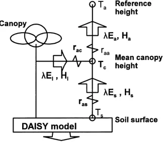
The sparse crop energy balance is described as follows, refer to Fig. 1.
Sensible heat flow between mean source height and reference height
Ha =ρcp Tc−Ta
raa (1)
Sensible heat flow between leaf surface and mean source height
Hl=ρcp Tl−Tc
Fig. 1. Schematic representation of resistance network and energy fluxes for the two-source SVAT component of the DAISY model. Aerodynamic resistances ras, racand raa as well as energy fluxes λE and H with indices s, l and a are defined between mean source height and soil, leaf, and reference height, respectively. Ts, Tcand Taare defined as temperatures at soil surface, mean canopy height and reference height, respectively.
Sensible heat flow between soil surface and mean source height
Hs=ρcp Ts−Tc
ras
(3)
Latent heat flow between mean source height and reference height
λEa=λ ec−ea
raa
(4)
Latent heat flow between leaf surface and mean source height
λEl=λ e∗l −ec rsc+rac
(5)
Latent heat flow between soil surface and mean source heightλEs is calculated in DAISY as the sum of upward flowing water from the soil matrix below and evaporation from eventual ponded water. It is as-sumed that the lateral flux between the soil and the mean canopy source height is negligible, i.e. water re-leased at the soil surface is transported without lateral loss to the mean canopy height node. In Eqs. (1)–(5), Ta, Tc, Tland Ts(K) are temperatures of air, in-canopy at mean source height, leaf and soil surface, respec-tively, and ea, ec, es (kg m−3) are water vapor con-tents at reference height, canopy mean source height and soil surface. It is assumed that stomatal air space
in the leaves is at 100% humidity, thereforee∗l is sat-urated vapor pressure at the leaf surface. All fluxes are in W m−2. Resistances raa, ras, racand rsc(s m−1) are defined in Eqs. (17), (18), (22) and (24), respec-tively, and λ is latent heat of vaporization of water (J kg−1). Conservation of fluxes through the canopy yield Eqs. (6) and (7)
Conservation of sensible heat
Ha−Hl−Hs =0 (6)
Conservation of latent heat
λEa−λEl−λEs=0 (7)
Conservation of energy for the plant canopy leads to
λEl+Hl=Al (8)
and for the soil surface
λEs+Hs=As (9)
Furthermore, as mentioned above, it is assumed that the stomatal air space in the leaves is at 100% and that this humidity (kg m−3) is a function of the leaf surface temperature
el∗=e∗a+∆(Tl−Ta) (10)
where ∆ is the slope of the saturation function for water vapor at Ta.
Aland Asin Eqs. (8) and (9) is energy that must be transmitted as sensible and latent heat into the air from the plant canopy and the soil surface, respectively, expressed in Eqs. (11) and (12)
Al=Rn(1−e−kL) (11)
and
As=Rn−kL−G (12)
is thus estimated from standard meteorological data: global radiation Si, air temperature Ta, vapor pressure ea and from relative duration of sunshine nsun. The longwave component is calculated by means of the Brunt (1932) equation (Rosenberg et al., 1983)
Ld−Lu=σ (Ta4(b1−b2p(ea))(b3+b4nsun)) (14) where air temperature Ta is in K, ea in kPa, bi are constants (b1 = 0.53, b2 = 0.0065, b3 = 0.1 and b4 = 0.9) and σ is the Stefan–Boltzmann constant. The relative duration of sunshine nsun is derived by rewriting the Prescott (1940) formula
Si =(ap+bpnsun)Sex (15) where Si is measured global radiation and Sexis the extraterrestrial radiation, a function of latitude and time of year, and ap and bp are site specific coeffi-cients. For the Danish Foulum location at 56◦30′N an average of the (daily) values found at DeBilt (52◦N, Kohsiek, 1971, unpublished) and Matanuscka-Anchorage, Alaska (61◦N, Baker and Haines, 1969) were used (references from Brutsaert (1982), p. 135), i.e. ap = 0.21 and bp =0.50. The phase difference in calculated extraterrestrial radiation and measured global radiation at solar and local time, respectively, is accounted for. G is calculated from Tsand a DAISY calculated upper soil temperature, T0
G=kh Ts−T0
1z (16)
where1z is depth of the upper soil layer and khis ther-mal conductivity of that layer returned by the DAISY model.
Eqs. (1)–(3) are substituted in Eq. (6), Eqs. (4) and (5) in Eq. (7) and Eqs. (11) and (12) in Eqs. (8) and (9), respectively. Then a linear system of five equations (Eqs. (6)–(10)), and five unknowns, Ts, Tc, Tl, ecand e∗l is obtained and solved using a Gauss–Jordan elim-ination. For each time step the involved resistances in the linear equation system are computed using Eqs. (17)–(29). Then, sensible and latent heat fluxes can be calculated by back substitution in Eqs. (1)–(5).
2.4. Network resistances
In unstable (temperature lapse) conditions, vertical motions are enhanced by buoyancy, effectively reduc-ing the aerodynamic resistance raa(Thom, 1975). This
can be accounted for by applying a stability correction factor based on the Businger–Dyer profiles (Dyer and Hicks, 1970; Dyer, 1974; Businger, 1988). Eq. (17) including the stabilityψ functions ψm andψh, de-fined for unstable conditions in Paulson (1970) and for stable conditions in Webb (1970), is applied by, e.g. Dolman (1993)
where h is vegetation height (m), d is displacement height (m), z0 is roughness length (m), uf is friction velocity (m s−1), zref is reference height (usually 2 m) and n is an eddy decay coefficient with a typical value of about 2.5. K(h) is an eddy diffusion coeffi-cient and defined in Eq. (19). The stability functions ψm∗ and ψh∗ are defined as ψm∗ = ψm(zref/Lo)− ψm(h/Lo)andψh∗ = ψh(zref/Lo) − ψh(h/Lo) in which Lo is the Obukhov stability length. Stability conditions between canopy mean height and reference height are here evaluated by the Richardson number Ri (Thom, 1975), unstable whenRi<0 and stable when Ri >0. It is commonly assumed (similarity hypoth-esis), that under fully forced convection conditions a single canopy aerodynamic resistance term, raa, rather than separate aerodynamic resistances for vapor and heat flow, rav and rah, can be used to calculate both latent and sensible heat fluxes, i.e.raa =rav = rah (Thom, 1975). Nichols (1992) derived ravand rah sep-arately from measured latent and sensible heat fluxes, respectively, by the Bowen ratio method above 0.75 m high sparsely vegetated shrubs in west central Nevada, USA. It was found that ravgenerally was one order of a magnitude higher than rah. Under the conditions at Foulum for 1997 it is assumed that the similarity hy-pothesis is valid until derived values from eddy covari-ance measurements become available for verification. Resistance between soil surface and canopy air, ras, is derived by Choudhury and Monteith (1988)
ras = he αk αkK(h)
(e−αkzs0/ h−e−αk(d+z0)/ h) (18) and the eddy diffusion coefficient K(h)
K(h)= κ
2u(h−d) ln((zref−d)/z0)
whereαk is attenuation coefficient of eddy diffusiv-ity through sparse canopy set to 2.0,zs0(=10−2m) is roughness length for the soil surface,κis the von Kár-máns constant (=0.41), u is wind speed at reference height and the rest previously defined. In common with Choudhury and Monteith (1988) and Shuttleworth and Gurney (1990) d and z0 are calculated as functions of leaf area index derived from second-order closure theory (Shaw and Pereira, 1982), yielding Eqs. (20) and (21) in which cd is the mean drag coefficient for a leaf, set to 0.05 (Shuttleworth and Gurney, 1990)
d =1.1hln(1+(cdL)0.25) (20)
The aerodynamic resistance between leaves and mean source height is defined by Jones (1983) and Choud-hury and Monteith (1988)
rac= αu
where u(h) is wind speed at h
u(h)=u coefficient for wind speed.
Finally, canopy resistance rsc is parameterized fol-lowing Dickinson (1984), Jarvis (1976) and Noilhan and Planton (1989) by using four constraint functions F1to F4and taking into account the physiology of the vegetation as applied by, e.g. Bougeault (1991) and Tourula and Heikinheimo (1998)
rsc= r min s
L (F1F2F3F4)
−1 (24)
where F1 is a function related to solar radiation and here parameterized following Dolman et al. (1991)
F1=
Si(T +Si)−1
1000(100+T )−1 (25)
where T is taken to be 250 W m−2 as optimized for oats in Dolman (1993).
The response of stomata to changing ambient hu-midity has been the subject of some controversy (Monteith, 1995a; Lhomme et al., 1998) and it has been proposed that stomata respond to the rate of transpiration rather than air humidity per se (Mott and Parkhurst, 1991). However, as there are uncertainties as how to upscale alternative constraint formulations as proposed by Monteith (1995b) from leaf to canopy, the Lohammar et al. (1980) environmental function is applied based on the findings that in many species, the stomatal resistance increases as the relative humidity decreases, i.e. as the leaf-to-air water vapor concen-tration difference increases (Turner, 1991), thus
F2=(1+ζ (e∗a−ea))−1 (26) using the value of 0.57 kg−1m3 for ζ, applied by Verma et al. (1993) for tall grass.
Although many parameterizations of stomatal resis-tance neglect the influence of ambient air temperature (see Lhomme et al. (1998) for a review) it has earlier been stated, e.g. Dickinson (1984), that stomatal re-sistance usually shows a decrease with increasing air temperature to a maximum value and then an increase at still higher ambient temperatures. This temperature optimum varies with species and can be increased by growth at high temperatures and vice versa. F3related to air temperature (Dickinson, 1984)
F3=1−ξ(Tref−Ta)2 (27)
whereξ =0.0002 K−2(Jarvis, 1976). Tref is a ‘refer-ence temperature’ (Noilhan et al., 1991) or optimum temperature as explained above (Turner, 1991) set to 298 K by Dickinson (1984).
Stomatal resistance increases as the soil dries, where soil water status influences stomatal conductance ei-ther through its influence on leaf water potential or by changes in the level of phytohormones produced by roots in response to soil dehydration. These processes are represented by the F4function taking account of water stress (Bougeault, 1991)
F4= θ−θwilt θc−θwilt
(28)
soil moisture content θ is calculated as an average of DAISY simulated water content at nodes within 0–100 cm.
The minimum resistance rcmin, i.e. rsmin/L in Eq. (24) is the parameter of interest for linking energy balance modeling, e.g. latent heat flux (evapotranspi-ration), to remote sensing data. However, as such data is not yet available for this study, minimum canopy resistance is estimated from rc in Eq. (29) (Allen et al., 1989; FAO, 1990)
rc= rday 0.5L =
200
L (29)
where rday is the average daily (24 h) stomatal resis-tance of a single leaf. Sellers et al. (1992a,b) estimated rcmin to be between 40 and 120 s m−1 for crops, cor-responding to LAI values from 5 to 1.7, respectively, in Eq. (29).
3. Study area and 1997 field campaigns
Field scale data for the RS-model project was collected at selected sites with agricultural crops at the Research Centre Foulum (RCF, 56◦30′N, 9◦36′E, altitude 45 m above sea level) in Jutland, Denmark. For the plot-scale study here focus was on a winter wheat crop. Height of the crop throughout the grow-ing season varied from 0.31 m (16 May), 0.41 m (26 May), 0.70 m (9 June), 0.80 m (24 June), 0.87 m (30 June) and 0.85 m until 8 August. Schjønning (1992) investigated the soils surrounding RCF and found for most of the profiles a rather homogeneous distribution of texture with depth. Soil content of clay generally increases from 7% in the topsoil to about 10–15% in the deepest part of the profile. The fine sand fraction (20–200mm) was found to make up about half the
particles in all depths. Meteorological data including radiation, precipitation, air humidity, air temperature and wind profiles, as well as water and carbon dioxide fluxes by means of eddy covariance equipment have been monitored at a winter wheat and spring barley site. Canopy related measurements such as spectral reflectance, leaf angle distribution, cover fraction, leaf area index, biomass and water content were specifically designed for accommodating the study of combining crop modeling and remote sensing. In addition soil moisture at various levels was measured
by means of time domain reflectometry (TDR) using horizontal and vertical probes. Data on soil tempera-ture and ground heat fluxes were also collected.
3.1. Meteorological data
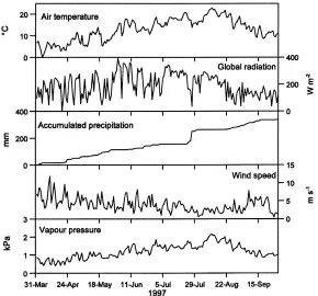
During the 1997 experiment all relevant meteoro-logical data was measured locally at the winter wheat site, see Fig. 2, and was used as forcing data for the DAISY model. However, during the ‘spin-up’ period prior to the 1997 campaign meteorological data from a nearby climate station (distance approximately 1 km) at the Foulum Research Centre is applied. Since the crop in question is a winter wheat, the ‘spin-up’ period was from June 1996 to approximately the beginning of April 1997 when some of the field campaign measure-ments were initiated. Missing local values from the climate mast at the winter wheat site were replaced by data from the nearby Foulum climate station. On-site precipitation data, available during the period of inter-est, was used for simulation purposes. Applied time step was 1 h.
3.2. Soil moisture measurements
Continuous soil profile measurements of water con-tent by TDR using single horizontal probes at 5, 10, 15, 20, 30, 40 and 50 cm on half hourly basis were compiled for the period 14 May to 8 August and av-eraged to hourly values. Soil water content by verti-cally inserted TDR probes for depths 0–20, 0–50 and 0–100 cm, were also available for the same period. The applied TDR system includes a 1502B/C Tektronix ca-ble tester (Tektronix Inc., Beaverton, OR) operated by a portable PC, a TSS 45 Tektronix multiplexer, inter-face electronics (Thomsen and Thomsen, 1994), and two wire TDR probes. Measured dielectric constants by the Tektronix cable tester were converted to volu-metric water content by the Topp et al. (1980) equa-tion. The software used for the analysis of TDR traces is discussed by Thomsen (1994).
3.3. Energy flux measurements
Fig. 2. Daily averaged meteorological variables at winter wheat plot from April to September 1997.
Instruments were mounted on a mast at a height of 2.5 m.
The eddy covariance and meteorological station was placed close (50 m) to the northern edge of the long and flat field of winter wheat. Fetch conditions to the N and NE of the station were considered inadequate due to the presence of a farm surrounded by tall trees (min-imum distance 135 m) and a forest edge (min(min-imum distance 290 m). Therefore, a bad fetch sector was de-fined comprising 129◦ to the N and NE of the sta-tion. The positive fetch sector, comprising 231◦, was to the W, S and SE of the station. Borders of the field were windbreaks (3–5 m high) situated at minimum and maximum distances of 200 and 750 m from the station, respectively. Fetch conditions were adequate throughout the day on 12 June, 19–21 June, 25–29 June, 9–23 July, and 5–7 August 1997. The closure of the energy balance (Rn−B−G−H−λE∼0) was generally not good. A regression of heat fluxes (H +λE) versus available energy (Rn−G), using all available 30 min concurrent measurements, yielded (H+λE)=0.71(Rn−G)+5 W m−2(R2=0.87). A
similar regression that included only data on days with a good fetch as defined above, produced (H+λE)= 0.70 (Rn−G)+5 W m−2 (R2 = 0.90), indicating that the closure problems were not related to fetch requirements. This leaves some 30% of the available energy to be accounted for by photosynthesis, canopy energy storage and measurement errors. The compo-nents whose order of magnitude could be evaluated were analyzed as described below.
The measurements of latent heat flux were evalu-ated by comparing to changes in water content mea-sured using the automated TDR station. Over periods with no rainfall, the difference from start to end in water content in the top 50 or 100 cm soil (eight repli-cates of each probe length) equals the amount of wa-ter lost as soil evaporation and crop transpiration to the atmosphere. We assume, in agreement to model predictions, that there is no significant drainage from the soil profile during such dry intervals. During the period 10–13 June 1997, the accumulated amount of water lost to the atmosphere according to the eddy correlation measurements was 11 mm, while the water content decline recorded by the 50 and 100 cm TDR probes corresponded to 11 and 13 mm of water, re-spectively. During the equally short dry period 18–20 June 1997, latent heat loss was equivalent to 9 mm of water, while the 50 and 100 cm TDR probes recorded water deficits of 9 and 12 mm, respectively. 9–23 July 1997 was a long dry spell. Observed water depletion during this period in the 0–50 and 0–100 cm soil depth was 49 and 69 mm, respectively. Accumulated latent heat loss during the dry spell was equivalent to 45 mm of water. Since the root zone of the wheat crop proba-bly exceeded 50 cm in July, and since we assume the TDR technique to be accurate in estimating relative changes in soil water content, the results indicate that eddy covariance estimates of latent heat flux could be underestimated in July.
4. DAISY model simulations
The model was set up to simulate on hourly basis from 1 June 1996 to 31 December 1997. Meteoro-logical forcings (global radiation, air temperature, air humidity, precipitation and windspeed) were retrieved from the RCF climate station using standard equip-ment. During the campaign period local forcing data were used whenever available as explained previously. The soil profile was partitioned in 20 compartments with discretization size varying from 2.5, 5 and 10 cm in the upper 75 cm to 10, 15, 20, 30 cm in the lower 75–200 cm. The hydraulic properties were parameter-ized following the Brooks and Corey (1964) model for soil water characteristics and the Mualem (1976) model for unsaturated conductivity. No soil profile measurements were conducted at the winter wheat site
for laboratory analyses, so hydraulic properties were estimated from previously performed profile analyses from adjacent locations. Brooks and Corey parameters were determined from an average of three soil profiles at four depth intervals: 0–32.5, 32.5–52.5, 52.5–100, and 100–230 cm. In the absence of locally measured hydraulic data and aware of the fact that large spa-tial variations in soil physical characteristics probably occur, Brooks & Corey parameters were adjusted to obtain good agreement between simulated and TDR measured soil moisture content for 0–0.2, 0–0.5 and 0–1.0 m. The saturated hydraulic conductivity is cal-culated as a logarithmic average of the three profiles for each horizon. Surface albedo for calculation of net radiation in Eq. (13) is estimated from measured in-coming and reflected radiation in 640–660 nm (red) using Skye SKR 1800 equipment during June, July and most of August. The mean value is 0.2 with a slight decreasing tendency from June to August. The winter wheat crop has been sampled several times during the growing season for crop development measurements like leaf area index, dry matter content and canopy height. LAI measurements for green, semigreen and yellow leaves by means of scanning in the laboratory have been supplemented by LAI2000 (Li-Cor) data for total LAI. Winter wheat was sown in September 1996 and harvested in August 1997. Application of both inorganic and organic (pig slurry) fertilizer are in accordance with recommended amounts (Plantedi-rektoratet, 1997/1998).
4.1. Simulation results
4.1.1. Net radiation
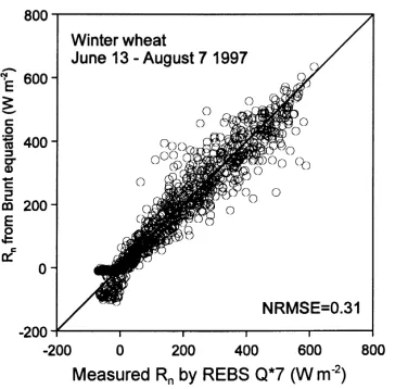
Fig. 3. Net radiation estimated using the Brunt equation vs. mea-sured net radiation.
ranging from 6 to 20%. In this study the normal-ized root mean square error (NRMSE) defined as
p
((Rsim
n −Robsn )2/n), i.e. RMSE, divided by the mean of Rnobs is 0.36 for day- and night-time val-ues and 0.25 for day valval-ues only, defined by Si > 10 W m−2, for the period 13 June to 7 August on hourly basis. Sensitivity analyses suggest that the best agreement as compared to the Q∗7 measurements (NRSME=0.31, Fig. 3) is obtained when the param-eter nsunin Eq. (14) is equal to zero, corresponding to full cloudiness, during night-time and estimated from Eq. (15) for day-time periods. The latter approach was therefore adopted for this study.
4.1.2. Crop development simulation
DAISY simulated crop development was evaluated against measured leaf area index and dry matter con-tent. Modeled LAI showed a too fast development in May compared to measured green LAI (GLAI) as de-termined in the laboratory (Fig. 4a, below). During June and July modeled LAI was slightly higher than measured GLAI. Simulated total dry matter content compared very well to measured total dry matter, i.e. green and dead material (Fig. 4a, top). Sub samples of dry matter content fractioned after stem, leaf and ears (Fig. 4b) were also in good agreement with mod-eled data. Simulated nitrogen content (not shown here) appeared to be close to values sampled from a field nearby with the same crop and fertilizer treatment.
Fig. 4. (a) Simulated (—) and measured (d) total winter wheat dry matter content and green LAI. (b) Simulated (—) and measured (d) winter wheat fractions.
4.1.3. Soil water modeling
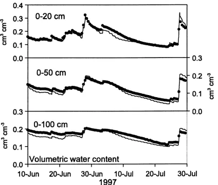
Fig. 5. Volumetric soil moisture content measured by time domain reflectometry (d) and simulated by the DAISY model (—) for 10 June to 30 July 1997.
this study is not modeling of soil water dynamics, it has not been attempted to optimize agreement between simulated and TDR measured soil moisture content for each horizontal level, nor to test model performance for other periods than the calibration period.
4.1.4. Energy balance modeling
Simulation of energy fluxes was performed for the period of 13 June to 7 August, when eddy covariance data was available. Bare soil evaporation contribution to latent heat flux is assumed to be negligible under full canopy conditions, but constitutes an increasing part with decreasing LAI. The relative importance of the rcmin parameter, amenable to RS data, is closer examined by substitution of rcmin −50%, rcmin and rcmin+50% in Eq. (24) for computation of canopy re-sistance rscfor subsequent use in Eq. (5) for simulation of latent heat flux from leaf surface to mean source height. This is demonstrated in Fig. 6 (lower graph), where rsc, moderated by the environmental constraint functions in Eqs. (24)–(28), is modeled for 18 and 19 June. From Fig. 6 (upper graph) it is clear that given the same environmental constraints, the value ofrcmin, as potentially sensed by RS data, is important for a correct modeling of latent heat flux through rsc in Eq. (24). However, it must be borne in mind that a correct specification of stress functions, which may be site-specific to a high degree, are at least equally
Fig. 6. Simulated (—) and measured (d) latent heat fluxes (λE) for different canopy resistance (rsc) values. Lower graph: rsc (—) as calculated from minimum canopy resistance,rmin
c in Eq. (24), rsc fromrmin
c +50% (m) and rsc fromrcmin−50% (.). Upper graph: largest simulatedλE for smallest rsc value and vice versa.
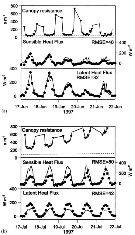
un-Fig. 7. (a) Simulated (—) and measured (d) energy fluxes for 17–22 June. Upper graph: stressed (.) and unstressed (- - -) canopy resistance, rsc and rmin
c , respectively. Note that the very high stressed canopy resistance values during night-time are truncated. (b) Simulated (—) and measured (d) energy fluxes for 17–22 July. Upper graph: stressed (.) and unstressed (- - -) canopy resistance, rscandrmin
c , respectively. Note that the very high stressed canopy resistance values during night-time are truncated.
derestimated. The low simulated fluxes are due to an increased control by the environmental functions, as mentioned before. Although the hydraulic parameters in the F4function were derived from actual field data and therefore physically based, there is little doubt that this function overestimated the water stress effect and needs improving or an alternative parameterization.
Fig. 8. Simulated (—) and measured (d) latent heat fluxes and simulated 0–50 cm soil moisture content, SMC (- - -). The periods 17–22 June (no water stress) and 17–22 July (water stress) are represented by top and bottom graph, respectively.
4.2. Potential link to remote sensing data
need to sense plant physiological development at this scale and use this information in simulation of surface energy fluxes.
5. Concluding remarks
The soil plant system simulation model DAISY extended by a two source resistance network for modeling energy balance processes for agricultural crops was presented. A two-source approach explic-itly accounts for bare soil evaporation and is therefore more generally applicable under different vegetation stages. The resistance approach for modeling sur-face energy fluxes provides a link to remotely sensed data through the unstressed canopy resistance rcmin upscaled by means of LAI. A simplified represen-tation of rcmin was applied as no remotely sensed data is yet available. A Jarvis–Stewart formulation for coupling the (actual) canopy resistance to rcmin by means of environmental constraint functions was implemented. Crop dry matter content and leaf area index are modeled adequately. Modeled soil water content, based on a Brooks & Corey parameterization, from 0 to 20, 0 to 50 and 0 to 100 cm were cali-brated satisfactorily against measured TDR values. Simulated and observed energy fluxes were generally in good agreement when water supply in the root zone was not limiting. With decreasing soil moisture content during a longer drought period, modeled la-tent heat flux was lower than observed, calling for both improved parameterization of environmental controls and for an improved estimation of the rcmin parameter. The latter can potentially be estimated at landscape scales by means of remote sensing data, which should lead to improved modeling of surface energy fluxes especially in areas where no ground based information on vegetation development is available.
List of symbols
Al available energy at leaf surface (W m−2)
As available energy at soil surface (W m−2) b1, b2, coefficients in Brunt equation
b3, b4
cd mean drag coefficient for a leaf cp specific heat of air at constant
pressure (J kg−1K−1)
d displacement height of vegetation (m) ea (measured) water vapor content at
reference height (2 m) (kg m−3)
ea∗ saturated water vapor content at reference height (2 m) (kg m−3)
ec water vapor content at mean source height (kg m−3)
el∗ saturated water vapor content at leaf surface (kg m−3)
Fi,i=1,environmental constraint functions of . . . ,4 Jarvis–Stewart type equation for rsc G ground heat flux (W m−2)
H sensible heat flux (W m−2)
Ha sensible heat flux from mean source to reference height (W m−2)
Hl sensible heat flux from leaf to mean source height (W m−2)
h vegetation height (m)
k extinction coefficient in Beer’s law type of equation
kh thermal conductivity of soil (W m−1K−1)
L leaf area index (m2m−2) LAI leaf area index (m2m−2)
Ld downwards longwave radiation (W m−2) Lo Obukhov stability length (m)
Lu upwards longwave radiation (W m−2) n eddy decay coefficient
nsun relative duration of sunshine (in Brunt equation)
Ri Richardson number Rn net radiation (W m−2)
raa aerodynamic resistance between canopy and reference height (s m−1)
rac boundary layer resistance of vegetative elements in canopy (s m−1)
rah aerodynamic resistance for sensible heat flow (s m−1)
ras aerodynamic resistance between soil surface and mean source height (s m−1) rav aerodynamic resistance for vapor flow
(latent heat) (s m−1)
rcmin minimum canopy resistance (s m−1) rday average daily (24 h) stomatal resistance of
single leaf (s m−1)
rsc bulk stomatal resistance of the canopy (s m−1)
rsmin minimum stomatal resistance (s m−1) Si global radiation (W m−2)
T coefficient in F1(W m−2)
Ta air temperature at reference height (measured) (K)
Tc canopy temperature at mean source height (K)
Tl leaf temperature (K)
Tref reference/optimum temperature in F3(K)
Ts soil temperature (‘skin’ temperature) (K)
Tsurf ‘bulk’ surface temperature (K) T0 soil temperature at depth1z simulated
by DAISY (K)
u windspeed at reference height (measured) (m s−1)
u(z) windspeed at height z (m s−1)
w average leaf width in equation for rac (m) x parameter in Businger–Dyer equations
argument
Y psychrometric ‘constant’ (h Pa K−1) z0 canopy roughness length (m) zs0 roughness length for the soil
surface (m)
zref reference height (2 m) (m)
Greek letters
α albedo
αk attenuation coefficient of eddy diffusivity through sparse canopy
αu attenuation coefficient of wind speed ∆ rate of change of absolute humidity with
temperature (kg m−3K−1) 1z soil depth (m)
ζ coefficient in F2(kg−1m3) κ von Karm´ ans constant´
λ latent heat of vaporization of water (J kg−1)
λE latent heat flux (W m−2)
λEa latent heat flux from mean source to reference height (W m−2)
λEl latent heat flux from leaf to mean source height (W m−2)
λEs latent heat flux from soil to mean source height (W m−2)
ψh stability correction function for sensible heat
ψh∗ derivedψh
ψm stability correction function for momentum
ψm∗ derivedψm
ρ density of air (kg m−3)
σ Stefan Boltzmann’s constant (W m−2K−1) θ soil water content simulated by DAISY
(cm3cm−3)
θc soil water content at ‘field capacity’ (cm3cm−3)
θwilt soil water content at ‘wilting point’ (cm3cm−3)
ξ coefficient in F3(K−2)
Acknowledgements
The RS-Model research program within the frame-work of the Earth Observation Program is funded by the Danish Space Board Committee, the Danish Agricultural and Veterinary Research Council and the Danish Technical Research Council. Per Abrahamsen (Danish Informatics Network in the Agricultural Sci-ences) is greatly acknowledged for his help on DAISY programming and technical advice.
References
Allen, R.G., Jensen, M.E., Wright, J.L., Burman, R.D., 1989. Ope-rational estimates of evapotranspiration. Agron. J. 81, 650–662. Asrar, G., Fuchs, M., Kanemasu, E.T., Hatfield, J.L., 1984. Esti-mating absorbed photosynthetic radiation and leaf area index from spectral reflectance in wheat. Agron. J. 76, 300. Baker, D.G., Haines, D.A., 1969. Solar radiation and sunshine
duration relationships in the North-Central region and Alaska. Tech. Bull. No. 262, University of Minnesota, Agric. Exp. Station, 372 pp.
Baldocchi, D., Meyers, T., 1998. On using eco-physiological micrometeorological and biochemical theory to evaluate carbon dioxide water vapor and trace gas fluxes over vegetation: a perspective. Agric. For. Meteorol. 90, 1–25.
sensing approach under clear skies in Mediterranean climates. Thesis Landbouwuniversiteit Wageningen.
Bougeault, P., 1991. Parameterization schemes of land-surface processes for mesoscale atmospheric models. In: Schmugge, T.J., André, J.C. (Eds.), Land Surface Evaporation: Measure-ment and Parameterization. Springer, Berlin.
Brooks, R.H., Corey, A.T., 1964. Hydraulic properties of porous media. Hydrology Paper no. 3, Colorado University, Fort Collins, CO, 27 pp.
Brunt, D., 1932. Notes on radiation in the atmosphere. Q.J.R. Meteorol. Soc. 58, 389–420.
Brutsaert, W., 1982. Evaporation into the atmosphere. Theory, History, and Applications. Reidel Publishing Company, Dordrecht/Boston/London, 1982.
Businger, J.A., 1988. A note on the Businger–Dyer profiles. Boundary-Layer Meteorol. 42., 145–151.
Chauhan, N.S., 1997. Soil moisture estimation under a vegetation cover. Combined active passive microwave remote sensing approach. Int. J. Remote Sens. 18 (5), 1079–1097.
Choudhury, B.J., Monteith, J.L., 1988. A four-layer model for the heat budget of homogeneous land surfaces. Q.J.R. Metorol. Soc. 114, 373–398.
Dickinson, R.E., 1984. Modeling evapotranspiration for three-dimensional climate models. Climate Processes and Climate sensitivity. Geophys. Monogr. No. 29, Am. Geophys. Union, pp. 58–72.
Diekkrüger, B., Söndgerath, D., Kersebaum, K.C., McVoy, C.W., 1995. Validity of agroecosystem models. A comparison of results of different models applied to the same data set. Ecol. Model. 81, 3–29.
Dolman, A.J., 1993. A multiple-source land surface energy balance model for use in general circulation models. Agric. Meteorol. 65, 21–45.
Dolman, A.J., Gash, J.H.C., Roberts, J.M., Shuttleworth, W.J., 1991. Stomatal and surface conductance of tropical rainforests. Agric. For. Meteor. 54, 303–318.
Dyer, A.J., 1974. A review of flux-profile relationships. Boundary-Layer Meteorol. 7, 363–372.
Dyer, A.J., Hicks, B.B., 1970. Flux-gradient relationships in the constant flux layer. Q.J.R. Meteorol. Soc. 96, 715–721. FAO, 1990. Expert consultation on revision of FAO methodologies
for crop water requirements. Annex V. FAO Penman-Monteith Formula.
Gamon, J.A., Penuelas, J., Field, C.B., 1992. A narrow-waveband spectral index that tracks diurnal changes in photosynthetic efficiency. Remote Sens. Environ. 41, 35–44.
Gillies, R.R., Carlson, T.N., Cui, J., Kustas, W.P., Humes, K.S., 1994. A verification of the ‘triangle’ method for obtaining surface soil water content and energy fluxes from remote measurements of the normalized difference vegetation index (NDVI) and surface radiant temperature. Int. J. Remote Sens. 18 (15), 3145–3166.
Halldin, S., Lindroth, A., 1992. Errors in net radiometry. Comparison and evaluation of six radiometer designs. J. Atmos. Oceanic Technol. 9, 762–783.
Hansen, S., Jensen, H.E., Nielsen, N.E., Svendsen, H., 1991. Simulation of nitrogen dynamics and biomass production in
winter wheat using the Danish simulation model DAISY. Fertilizer Res. 27, 245–259.
Hatfield, J.L., 1983. Evapotranspiration obtained from remote sensing methods. In: Hilled, D.E. (Ed.), Advances in Irrigation. Academic Press, New York, pp. 395–416.
Jacobs, C.M.J., 1994. Direct impact of atmospheric CO2 enrichment on regional transpiration. PhD thesis, Agricultural University, Wageningen.
Jarvis, P.G., 1976. The interpretation of the variations in leaf water potential and stomatal conductance found in canopies in the field. Phil. Trans. R. Soc. London Ser. B 273, 563–610. Jensen, C., Stougaard, B., Olsen, P., 1994. Simulation of nitrogen
dynamics at three Danish locations by use of the DAISY model. Acta Agriculturae Scandinavica, Section B. Soil Plant Sci. 44, 75–83.
Jones, H.G., 1983. Plants and Microclimate. Cambridge University Press, New York.
Kustas, W.P., 1990. Estimates of evapotranspiration with a one-and two-layer model of heat transfer over partial canopy cover. J. Appl. Meteorol. 29., 704–715.
Kustas, W.P., Prueger, J.H., Hipps, L.E., Hatfield, J.L., Meek, D., 1998. Inconsistencies in net radiation estimates from use of several models of instruments in a desert environment. Agric. For. Meteor. 90, 257–263.
Lhomme, J.-P., Elguero, E., Chehbouni, A., Boulet, G., 1998. Stomatal control of transpiration. Examination of Monteith’s formulation of canopy resistance. Water Resour. Res. 34 (9), 2301–2308.
Lohammar, T., Larsson, S., Lindner, S., Falk, S., 1980. FAST simulation models of gaseous exchange in Scots pine. Structure and function of northern coniferous forests — an ecosystem study. Ecol. Bull. 32, 505–523.
Makkink, G.F., 1957. Ekzameno de la formula de Penman. The Netherland J. Agric. Sci. 5, 290–305.
Monteith, J.L., 1965. Evaporation and the environment. Symp. Soc. Expl. Biol. 19, 205–234.
Monteith, J.L., 1977. Climate and the efficiency of crop production in Britain. Philos. Trans. R. Soc. London Ser. B 281, 277–294. Monteith, J.L., 1995a. A reinterpretation of stomatal responses to
humidity. Plant Cell Environ. 18, 357–364.
Monteith, J.L., 1995b. Accommodation between transpiring vegetation and the convective boundary layer. J. Hydrol. 166, 251–263.
Moran, M.S., Jackson, R.D., Raymond, L.H., Gay, L.W., Slater, P.N., 1989. Mapping surface energy balance components by combining Landsat thematic mapper and ground-based meteorological data. Remote Sens. Environ. 30, 77–87. Mott, K.A., Parkhurst, D.F., 1991. Stomatal responses to humidity
in air and helox. Plant Cell Environ. 14, 509–515.
Mualem, Y., 1976. A new model for predicting the hydraulic conductivity of unsaturated porous media. Water Resour. Res. 12, 513–522.
Nichols, W.D., 1992. Energy budgets and resistances to energy transport in sparsely vegetated rangeland. Agric. For. Meteor. 60, 221–247.
satellite microwave radiometry, ISLSCP. In: Proceedings of an International Conference, Rome, Italy. ESA, SP-248, Paris, pp. 349–356.
Noilhan, J., Planton, S., 1989. A simple parameterization of land-surface processes for meteorological models. Mon. Wea. Rev. 117, 536–549.
Noilhan, J., et al., 1991. Some aspects of the HAPEX-MOBILHY programme. In: Wood, E.F. (Ed.), Land Surface/Atmosphere Interactions for Climate Modeling, Kluwer Academic Publi-shers, Dordrecht, pp. 31–62.
Ottlé, C., Vidal-Madjar, D., Cognard, A.L., Loumagne, C., Normand, M., 1996. Radar and optical remote sensing to infer evapotranspiration and soil moisture. In: Steward, et al. (Eds.), Scaling up in Hydrology Using Remote Sensing. Wiley, Chicester.
Paulson, C.A., 1970. The mathematical representation of windspeed and temperature profiles in the unstable atmospheric surface layer. J. Appl. Meteorol. 9, 857–861.
Petersen, C.T., Jørgensen, U., Svendsen, H., Hansen, S., Jensen, H.E., Nielsen, N.E., 1995. Parameter assessment for simulation of biomass production and nitrogen uptake in winter rape. Eur. J. Agron. 4, 77–89.
Plantedirektoratet, 1997/1998. Vejledning og skemaer. Ministeriet for Fødevarer, Landbrug og Fiskeri (in Danish).
Prescott, J.A., 1940. Evaporation from a water surface in relation to solar radiation. Trans. Roy. Soc. Australia 64, 114–125. Rosenberg, N.J., Blad, B.L., Verma, S.B., 1983. Microclimate: The
Biological Environment, 2nd Edition, Wiley, New York, 1983, 495 pp.
Schelde, K., Thomsen, A., Heidmann, T., Schjønning, P., Jansson, P.B.E., 1998. Diurnal fluctuations of water and heat flows in a bare soil. Water Resour. Res. 34 (11), 2919–2929.
Schjønning, P., 1992. Characterization of the area surrounding Research Centre Foulum (summary in English). Beretning nr. S 2229, 1992, landbrugsministeriet, Statens Planteavlsforsøg. Sellers, P.J., 1985. Canopy reflectance, photosynthesis and
transpiration. Int. J. Remote Sens. 6., 1335–1372.
Sellers, P.J., 1987. Canopy reflectance, photosynthesis, and transpiration. II. The role of biophysics in the linearity of their interdependence. Remote Sens. Environ. 21, 143–183. Sellers, P.J., 1991. Modeling and observing land–surface–
atmosphere interactions on large scales. In: Wood, E.F. (Ed.), Land–Surface–Atmosphere Interactions for Climate Modeling: Observations, Models and Analysis. Kluwer Academic Publi-shers, Dordrecht, 1991.
Sellers, P.J., Berry, J.A., Collatz, G.J., Field, C.B., Hall, F.G., 1992a. Canopy reflectance, photosynthesis, and transpiration. III. A reanalysis using improved leaf models and a new canopy integration scheme. Remote Sens. Environ. 42, 187–216. Sellers, P.J., Heiser, M.D., Hall, F.G., 1992b. Relations between
surface conductance and spectral vegetation indices at intermediate (15–100 km2) length scales. J. Geophys. Res. 97 (D17), 19033–19057.
Shaw, R.H., Pereira, A.R., 1982. Aerodynamic roughness over a plant canopy: a numerical experiment. Agric. Meteorol. 26, 51–65.
Shuttleworth, W.J., Gurney, R.J., 1990. The theoretical relationship between foliage temperature and canopy resistance in a sparse crop. Q.J.R. Meteorol. Soc. 116, 497–519.
Shuttleworth, W.J., Wallace, J.S., 1985. Evaporation from sparse crops — an energy combination theory. Q.J.R. Meteorol. Soc. 111, 839–855.
Smith, P., Smith, J.U., Powlson, D.S., Arah, J.R.M., et al., 1997. A comparison of the performance of nine soil organic matter models using datasets from seven long-term experiments. Geoderma 81 (1/2) 153–222.
Svendsen, H., Hansen, S., Jensen, H.E., 1995. Simulation of crop production, water and nitrogen balances in two german agro-ecosystems using the DAISY model. Ecol. Model. 81, 197–212.
Tenhunen, J.D., Geyer, R., Valentini, R., Mauser, W., Cernusca, A., 1999. Ecosystem studies, land-use, and resource management. In: Tenhunen, J.D., Kabat, P. (Eds.), Integrating Hydrology, Ecosystem Dynamics, and Biochemistry in Complex Landscapes. Wiley, Chicester.
Thom, A.S., 1975. Momentum, mass and heat exchange of plant communities. In: Monteith, J.L. (Ed.), Vegetation and the Atmosphere: Principles, Vol. I. Academic Press, London, pp. 57–109.
Thomsen, A., 1994. Program AUTOTDR for making automated TDR measurements of soil water content. SP Rep. 38, 17 pp. Danish Institute of Plant and Soil Science, Tjele, 1994 (available at [email protected]).
Thomsen, A., Thomsen, H., 1994. Automated TDR measurements. Control box for Tektronix TSS 45 relay scanners. SP rep. 10, 29, 29 pp. Danish Institute of Plant and Soil Science, Tjele, 1994 (available at [email protected]).
Topp, G.C., Davis, J.L., Annan, A.P., 1980. Electromagnetic determination of soil water content. Measurements in coaxial transmission lines. Water Resour. Res. 3, 574–582.
Tourula, T., Heikinheimo, M., 1998. Modelling evapotranspiration from a barley field over the growing season. Agric. For. Meteor. 91, 237–250.
Tucker, C.J., Holben, B.N., Elgin, J.H., Mcmurtrey, E., 1981. Remote sensing of total dry matter accumulation in winter wheat. Remote Sens. Environ. 11, 171–190.
Turner, N.C., 1991. Measurements and influence of environmental and plant factors on stomatal conductance in the field. Agric. For. Meteorol. 54, 137–154.
Verma, S.B., Sellers, P.J., Walthall, C.L., Hall, F.G., Kim, J., Goetz, S.J., 1993. Photosynthesis and stomatal conductance related to reflectance on the canopy scale. Remote Sens. Environ. 44, 103–116.
Wang, J.R., Shiue, J.C., Schmugge, T.J., Engman, E.T., 1989. L-band radiometric measurements of the FIFE test site in 1987/88. Presented at the AMS symposium on the First ISLSCP Field Experiment (FIFE), 7–9 February, Anaheim, CA, pp. 85–87.
Webb, E.K., 1970. Profile relationships: the log-linear range, and extension to strong stability, and extension to strong stability. Q.J.R. Meteorol. Soc. 117, 67–90.
Wessman, C.A., Cramer, W., Gurney, R.J., Martin, P.H., Mauser, W., Nemani, R., Paruelo, J.M., Penuelas, J., Prince, S.D., Running, S.W., Waring, R.H., 1999. Group report: remote sensing perspectives and insights for study of complex
landscapes. In: Tenhunen, J.D., Kabat, P., Wessman, C.A. (Eds.), Integrating Hydrology, Ecosystem Dynamics, and Biochemistry in Complex Landscapes. Wiley, Chicester.