THREE-DIMENSIONAL BUILDING RECONSTRUCTION USING IMAGES
OBTAINED BY UNMANNED AERIAL VEHICLES
Cornelius Wefelscheid, Ronny H¨ansch, Olaf Hellwich
Computer Vision and Remote Sensing Berlin University of Technology
Sekr. FR3-1, Franklinstr. 28/29, D-10587, Berlin, Germany (cornelius.wefelscheid, r.haensch, olaf.hellwich)@tu-berlin.de
KEY WORDS:UAVs, Photogrammetry, 3D Reconstruction, Sensor Orientation
ABSTRACT:
Unmanned Aerial Vehicles (UAVs) offer several new possibilities in a wide range of applications. One example is the 3D reconstruction of buildings. In former times this was either restricted by earthbound vehicles to the reconstruction of facades or by air-borne sensors to generate only very coarse building models. This paper describes an approach for fully automatic image-based 3D reconstruction of buildings using UAVs. UAVs are able to observe the whole 3D scene and to capture images of the object of interest from completely different perspectives. The platform used by this work is a Falcon 8 octocopter from Ascending Technologies. A slightly modified high-resolution consumer camera serves as sensor for data acquisition. The final 3D reconstruction is computed offline after image acquisition and follows a reconstruction process originally developed for image sequences obtained by earthbound vehicles. The per-formance of the described method is evaluated on benchmark datasets showing that the achieved accuracy is high and even comparable with Light Detection and Ranging (LIDAR). Additionally, the results of the application of the complete processing-chain starting at image acquisition and ending in a dense surface-mesh are presented and discussed.
1 INTRODUCTION
The automatic generation of accurate three-dimensional models is useful for a wide range of applications including robot guid-ance, computer-graphics, virtual reality, communication, and vi-sual inspection for example during industrial quality assessment. Especially the three-dimensional reconstruction of buildings is important due to its potential for the usage of 3D city models in city planning, damage assessment, monument conservation, ar-chitecture, and digital tourism.
Earthbound vehicles only move on the ground. Images captured by them can be used for the reconstruction of facades. The roof or concave structures cannot be imaged with reasonable effort. In contrast, conventional air-borne sensors are not able to model details at the facade. They help to determine the coarse shape of a building, but cannot model the whole building with a high de-gree of detail. UAVs combine the advantages of earthbound and air-borne sensors. They can exploit the whole three-dimensional space as long as it is free of obstacles. They allow for differ-ent imaging positions and therefore enable the acquisition of the whole object.
This paper proposes a complete and automatic processing chain, beginning with acquiring images over feature tracking, path esti-mation, and resulting in a dense three-dimensional surface model.
The Falcon 8 octocopter from Ascending Technologies is utilized as flight platform in this work. A high resolution consumer cam-era with a prime lens is used as imaging sensor. In the special case of gathering 3D information with a UAV of less than 5Kg heavy laser-scanning sensors cannot be employed and a light-weight camera is the only possibility.
The final 3D reconstruction is computed offline after image ac-quisition and follows the reconstruction process originally de-veloped for image sequences obtained by earthbound vehicles. Interest points within all images are found with the F¨orstner
op-erator (F¨ostner and G¨ulch, 1987) and described by SIFT (Lowe, 2004). Due to the low precision of the on-board GPS and IMU, the trajectory of the camera is computed only from images. For the best accuracy, an optimal set of images in the sense of view-ing angle and number of matches is selected for path estimation. An additional loop closure detection lead to robust and precise results. Bundle adjustment is applied as a final optimization step (Lourakis and Argyros, 2009). After path estimation, a dense point cloud is computed with a robust multi-view stereopsis ap-proach (Furukawa and Ponce, 2010). Finally, a Poisson surface reconstruction method (Kazhdan et al., 2006) fits a polyhedral mesh into the complete point cloud.
The described processing-chain computes all results fully auto-matically. Even image capturing is done automatically by the UAV for a precomputed path. The proposed method achieves precise results on different benchmark datasets. Furthermore, the capabilities of the whole processing chain are exemplary illus-trated by reconstructing a building from UAV image data.
2 RELATED WORK
Due to the large impact of three-dimensional building models and the high cost of generating them manually, the task of automati-cal building reconstruction was extensively addressed by the sci-entific community.
While air-borne data provide outline and shape of building roofs, ground based views are suitable for facade reconstruction. UAVs are theoretically able to capture data from all viewing positions. However, due to weight constraints it is not possible to mount a LIDAR sensor on a modern UAV. Merging of point clouds from different data sources is possible, but non-trivial especially if they are obtained by such different viewing positions as for ground-based and air-borne sensors. Even if LIDAR data is used for building reconstruction, optical images will still be needed for coloring and texturing the derived building models.
Image-based reconstruction methods offer a couple of advantages compared to LIDAR. Lasers are heavy and expensive, while light-weight high-resolution cameras are of considerably lower cost. Another reason for using cameras is the ease of acquiring im-age data. While a LIDAR system has to be operated by experts, image acquisition with cameras can be carried out by laymen. During data recording with a LIDAR sensor, the different posi-tions are precisely measured in order to merge the submaps to a global reconstruction afterwards. In the case of a structure from motion approach, this task is part of the reconstruction toolchain and automatically solved by the computer. Recent image-based reconstruction methods lead to robust and accurate 3D models that are comparable to those of LIDAR approaches (Strecha et al., 2008).
Different structure from motion approaches have been presented in the past. A quite popular approach, which works on inter-net photo collections such as flickr (Agarwal et al., 2009), is de-scribed in (Snavely et al., 2007). This method was accelerated by (Frahm et al., 2010) to deal with the same amount of images on a single computer. All approaches are mainly based on iteratively applying bundle adjustment. Within this work the number of nec-essary bundle adjustments is limited. Additionally, a new strat-egy to detect loop closures is presented. This approach achieves similar accuracy by lower computational costs. Nevertheless, the main focus is not on the calculation period, but the accuracy of the reconstruction.
3 HARDWARE
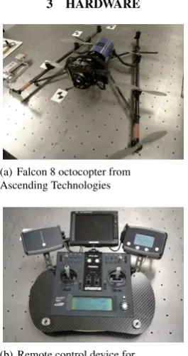
(a) Falcon 8 octocopter from Ascending Technologies
(b) Remote control device for human interaction
Figure 1: Hardware used for this work.
The Falcon 8 shown in Fig. 1(a) is used in this work. Eight rotors allow a safe landing even in the case of a serious failure of one motor during the flight. The weight of the UAV alone is 1.5 kg with an additional payload of 500 g. The maximal flight time is approximately 20 minutes, depending on the actual payload. Several sensors such as GPS, IMU, height sensor and compass are readily mounted on board to facilitate a stable and easy con-trollable flight.
Due to the included ground control software the used UAV is able to fly a fixed path using predefined GPS waypoints. However, law restrictions in Germany do not allow a fully automated flight. The user either has to steer the UAV manually or at least must be able to interrupt an automated flight at any time. Both can be accom-plished by the remote control shown in Fig. 1(b).
A high-resolution consumer camera from Panasonic (Lumix GF1) is used for image acquisition. The camera weighs only 285 g and therefore fulfills the payload constraint. It provides images of an resolution of 12.1 Megapixel with a 20 mm prime lens.
4 DATA ACQUISITION
The usage of UAVs enables image acquisition of objects from viewing positions, which are impossible to take up by earthbound vehicles. The flight path might be planned in advance with the flight control software. This shortens the flight time as well as the overall time in the field. This is important, since the time of operation is much stronger restricted for UAVs than for earth-bound vehicles.
The flight control software receives a set of waypoints. One way-point is described by a vector consisting of GPS coordinates (only taken for 2D positioning), height, horizontal orientation angle, and a vertical camera angle.
Images of the scene are acquired with a pre-calibrated high res-olution digital camera (see Section 3). The high resres-olution leads to a more accurate path estimation as well as a precise 3D recon-struction which is comparable to LIDAR systems (e.g. (Strecha et al., 2008)).
If the flight path is predefined, the images either will be taken at the waypoints or the continuous shooting mode of the camera will be utilized for a more dense image sequence. In the latter case, images are gathered with a frame rate of up to three images per second.
5 THREE-DIMENSIONAL BUILDING RECONSTRUCTION
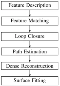
This section provides an overview over the processing chain used by this work to estimate a three-dimensional building model from previously acquired images. The subsequent subsection discusses the individual parts of the processing chain (shown in Fig. 2) in more detail.
Feature Description
Feature Matching
Loop Closure
Path Estimation
Dense Reconstruction
Surface Fitting
Figure 2: Flowchart of the toolchain.
The comparison of every feature point of one image with all feature points of all the other images would be time consum-ing. Therefore, Section 5.2 proposes a loop closure detection approach in order to determine a subset of the whole image se-quence which probably matches with a specific image.
From the set of matched image points, the external calibration of the image sequence is calculated. In particular, the precise path of the camera is determined. Details of the used path-estimation method are discussed in Section 5.3.
Once all camera positions are calculated, a dense point cloud is derived by utilization of the method described by (Furukawa and Ponce, 2010). A final step defines a closed surface constraint by the point cloud (Kazhdan et al., 2006). Both steps are briefly explained in Section 5.4.
5.1 FEATURE DETECTION and MATCHING
The proposed processing chain is universal and can be applied to a wide range of tasks concerning 3D-reconstruction from images. Nevertheless, the main objective of this work is the automatic generation of three-dimensional building models.
Like most man-made structures, images of buildings con-tain strong edges as dominant visual characteristics. Joints of edges lead to corner-like image regions. Those can be located with high accuracy within the image and their visual proper-ties are robust with respect to radiometric and geometric changes.
A common method to define interest points in images is SIFT (Lowe, 2004), which basically consists of two distinct parts, namely the detection and description of interest points. As shown in (Rodehorst and Koschan, 2006), F¨orstner points (F¨ostner and G¨ulch, 1987) detect corners in images with higher accuracy than the SIFT detector. For this reason, the well known SIFT descriptor and the F¨orstner interest point detector are combined in this work in order to produce a set of well located keypoints per image, where each keypoint is described by the
128-dimensional SIFT descriptor.
After keypoints are located and described in each image, they have to be matched between the different images. This means in particular to find all feature points in all images, that are a projection of the same three-dimensional point within the scene.
A keypoint of an imagefwill be assumed to match with a key-point in imagegif the euclidean distance between their descrip-torsD~fi andD~g
mis smaller than the distance to all other
descrip-tors in imagegand less than a pre-defined thresholdT (Eq.1).
Additionally, the ratio between the smallest and second smallest euclidean distance (the outlier distance (Brown et al., 2005)) has to be less than a thresholdR(Eq.2):
||D~fi −D~mg1||2 < T (1)
~
Dgm1= argmin
~ Dgj∈Dg
||D~fi −D~ g j||2
||D~if−D~ g m1||2
||D~if−D~gm2||2
< R (2)
~
Dgm2= argmin
~
Dgj∈Dg\D~g m1
||D~if−D~gj||2
In all experiments of Section 6 those thresholds are set to
T = 8000andR= 0.7.
Using this methodology, the keypoints of each image are com-pared with the keypoints of all of its predecessors until three suc-cessive images do not lead to a sufficient number of matches. A small percentage of strongly degraded images (e.g. due to motion blur) can thus be tolerated. Additional image pairs, that belong to potential loop closures, are matched. Their identification will be described in Section 5.2 in detail.
A subsequent evaluation of all feature pairs against a fundamental matrix prevents coarse errors. This filtering step does not detect all existing outliers. An additional trifocal filter is integrated after all images have been processed. For each image triplet that pos-sesses a high number of matches, a trifocal tensor is computed. All feature triplets are tested of consistency with the estimated tri-focal tensor. If the resulting error lies below a pre-defined thresh-old, the feature triplet will be accepted or rejected, respectively (Heinrichs and Hellwich, 2008). Features, that are only matched in one image pair, are discarded as well. The remaining features form a stable and nearly outlier free set of feature matches.
This set of features has to be further divided into subsets of fea-ture points that correspond to the same 3D point. If a feafea-turefi
has no matches with feature points within the predecessors of im-agei, a unique ID will be assigned to it. Otherwise, the ID of the predecessors of this feature is used. In the case that the prede-cessors of a feature have different IDs, the ID with the maximum count in the list of predecessors is assigned. Merging the IDs was tried, but it lead to a higher amount of mislabeled features.
After all features in an image are labeled, a simple consistency check is performed. If two features within one image have the same ID, the check fails and the ID will be rejected.
5.2 LOOP CLOSURE DETECTION
Depending on the actual path of the camera, the same part of the scene might be imaged multiple times. The more often a 3D point is observed, the more information about this point is avail-able, which can be used for a robust and more accurate estima-tion. This makes loop-closure detection essential for subsequent algorithms. The problem is defined as detecting, when the cam-era has returned to a previously visited position, where it acquired a similar image.
good recognition rate, where visual words are used to describe an image. One disadvantage of those approaches is the rather large computational load to build the tree and query an image.
This work proposes Variance Descriptor Analysis (VDA) as a new method to detect loop closures. Although this approach is less accurate than vocabulary trees, it is much faster.
Theoretically, it is possible to match all images according to the methodology discussed in Section 5.1. A loop will be identified if two images are likely to match each other. Of course the compu-tational costs to match one image with all of the previous images are to high. Instead, a method is used, which defines a set of matching candidates.
Two images will match, if many of their SIFT features match. A new descriptor is computed from all descriptors in one image. Given all128-dimensional SIFT descriptorsDfi in an imagef, the variance descriptorV~f
is defined as
~ Vf = 1
n−1
n
X
i=1
~
Dif−Df2 (3)
whereDfis the mean vector of all features in imagef.
Given one variance descriptor per image, a similarity matrixM between all images is calculated as the normalized inner product of two differentV~-vectors:
Mf,g=
~ Vf T·V~g
||V~f|| · ||V~g|| (4)
(a) Similarity matrixM (b) After thresholding
Figure 3: Similarity matrix for VDA.
Fig. 3(a) shows an exemplary similarity matrixMbased on real-world data. Values near the main diagonal are quite large. This is due to the fact that the data used in this work represents an or-dered image sequence and neighboring images have a high match-ing score. This effect is exploited to define a threshold as the mean similarity of the images already successfully matched as described in Section 5.1.
Fig. 3(b) shows the similarity matrix after applying the threshold. A standard matching procedure is applied to all remaining poten-tial matches, marked in black. Candidates with less matches than a predefined minimum are rejected. The global IDs are assigned as described in Section 5.1.
5.3 PATH ESTIMATION
The path estimation algorithm used in this work represents the whole camera sequence as graph that consists of two different kinds of nodes. While the first node type describes an image triplet, the second type contains only one single image (see Fig. 4). The graph contains all nodes previously created in the trifocal fil-ter step.
A node of the second type is connected with all triplet nodes that contain the image represented by this node. An image triplet node contains the relative orientations and scaling factors, which are shared by three cameras. The relative orientations are computed by the well known 5 point relative pose algorithm described by (Nist´er, 2004). The scaling factor is the distance between the second and the third camera. The distance between the first and second camera is set to1.0. Two triplet nodes share an edge if two of the three images are the same.
Each triplet node is optimized with bundle adjustment (Lourakis and Argyros, 2009). If the change, the bundle adjustment applies to a node, is too large in terms of the orientation of the cameras and the relative scale, the node will be rejected as unreliable.
0 1 2
0
1
2 0 1 3
0 2 3
1 2 3
3
Figure 4: Example graph illustrating the connection between triplets and cameras.
The great advantage of this procedure is the possibility to im-plement it in a highly parallel manner since each node can be treated separately. Once the graph is generated an optimal path through the graph is computed. For faster computation, the de-gree of each node is measured as local centrality measure instead of a global optimization (Opsahl et al., 2010). The node with the highest score is selected as root for further camera path propa-gation and the shortest path to each camera, ie. the second node type, is computed. This guarantees a limitation of the error made by propagating the camera position from one triplet to the next.
5 19 20
3 5 19 5 7 19 4 19 20 16 19 20 5 17 19 20 6 19 20 7 19 20 18 19 20 19 8 19 20 20 9 19 20 19 20 21 19 20 22 10 19 20
2 3 5 3 5 16 3
0 2 3 2
0 1 3 16 3 14 16
1 14 5 7 15
15
4 16 17 6 7 18 8 9 21 22 20 22 23 10 10 11 20
11 10 11 12 10 11 23
12 11 12 23 23
11 23 24
24 12 23 24
12 13 24
13
Figure 5: Spanning tree from the most central node to each camera for the Herz-Jesu-P25 sequence.
Finally, all camera positions are again optimized with the bundle adjustment method (Lourakis and Argyros, 2009). As shown in Fig. 5, the number of triplet nodes to reach a camera from the root node is reduced drastically in contrast to a sequential cam-era path propagation. This leads to a better approximation of the initial camera position and reduces the risk that the bundle adjust-ment terminates at a local minimum.
5.4 DENSE RECONSTRUCTION
The method proposed in (Furukawa and Ponce, 2010) is used to derive a dense point cloud. It does not depend on any initial-ization other than provided by the previous path estimation step, detects and disregards outliers automatically, is able to use an ar-bitrary number of images, and performs best on four of six bench-mark data sets discussed in (Seitz et al., 2006).
estimated by previous steps serve as input and are successively transformed into a set of image patches. A patchpis defined by the 3D coordinates of the centerc(p)and the orientation of the vectorn(p)orthogonal to the patch.
Features based on Harris- and Difference-of-Gaussians-operators are computed for each image in an initial matching step. Fea-ture points of different images will be matched if they lie near the epipolar line and are photometrically consistent, i.e. the nor-malized grey-scale correlation of their projection into the image planes is smaller than a threshold. Those matched feature points are triangulated and serve as initial set of sparse patches.
An expansion step generates new patchesp′in close proximity
to already defined image patchesp. Centerc(p′) and orienta-tionn(p′)are initialized consistently with patches in the neigh-borhood and optimized afterwards. A subsequent filtering step detects outliers based on visibility or photometric constraints. Those two steps are iteratively repeated until a sufficiently dense set of patches is defined.
A 3D surface of the whole scene is computed by a subsequent surface reconstruction step based on this patch model. The ap-proach proposed by (Kazhdan et al., 2006) is utilized for this aim. It expects a set of samplesP, where each samplep∈Pconsists of a center pointc(p)and an inward-facing normal vectorn(p). Those samples are assumed to lie on, or at least near, the surface of the unknown model.
Given this input, the method casts the surface reconstruction task as spatial Poisson problem, i.e. finding the scalar function χ whose gradient gives the best approximation of a vector field which is defined by the samples. For this purpose, a three-dimen-sional indicator function is computed, which is zero outside and one inside the model. An appropriate iso-surface of this function is used as the reconstructed surface.
The spatial and temporal complexity of the necessary calculations are proportional to the size of the reconstructed surface. Instead of using only a small local subset of points at a time, all points of the input set are used at once. This leads to a smooth and well defined surface with greater detail and higher accuracy than achievable with other methods.
6 RESULTS
The performance of the proposed processing chain is evaluated on three datasets including two different benchmarks as well as one dataset acquired by the system described in Section 3.
The benchmark datasets, namely Herz-Jesu-P25 and Castle-P30 provided by (Strecha et al., 2008), are used for a precise and com-parable accuracy evaluation. These datasets are not acquired by a UAV but prove the general accuracy of the proposed approach.
Along with the high-resolution images, the internal as well as the external orientation of the cameras are provided. The computed reconstruction is unique up to one scaling, three translation, and three rotation parameters. A transformation regarding these seven parameters is applied to the estimated cameras in order to trans-form them to the ground truth coordinate system.
The difference between ground truth and the results of the pro-posed method are illustrated in Figs. 6 and 7. A very low av-erage error of less than one centimeter for the Herz-Jesu-P25 dataset and three centimeter for the sparser Castle-P30 dataset is
0 5 10 15 20 25 30
camera index 0.00
0.01 0.02 0.03 0.04 0.05 0.06 0.07 0.08 0.09
distance [m]
Herz-Jesu-P25 Castle-P30 Castle-P30_Loop
Figure 6: Distance error from Herz-Jesu-P25 and Castle-P30 with and without loop closure.
0 5 10 15 20 25 30
camera index 0.00
0.02 0.04 0.06 0.08 0.10 0.12 0.14 0.16 0.18
angle [degree]
Herz-Jesu-P25 Castle-P30 Castle-P30-Loop
Figure 7: Angle error from Herz-Jesu-P25 and Castle-P30 with and without loop closure.
achieved. Since the camera in the Herz-Jesu-P25 dataset moves only along one direction, this dataset is dense enough, whereas the Castle-P30 dataset does a complete360degree rotation. More images are necessary to achieve a similar error on both datasets. The loop closure at the end of the sequence facilitates precise re-sults (see Figs. 6 and 7).
As shown in (Strecha et al., 2008) the accuracy of the posi-tion (3σ) is approximately around 1-2 cm for the Herz-Jesu-R23 ground truth dataset. A similar accuracy is assumed for the Herz-Jesu-P25 dataset, although its precision is not provided. The re-sults in Fig. 6 show, that the achieved error rate is within the3σ range of the reference data. The ground truth was produced with a LIDAR system, whose variance and the error rate are in the same range. Therefore, the discussed processing chain is able to provide results that are competitive with LIDAR systems in terms of accuracy.
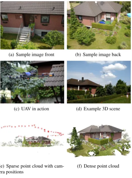
The last dataset is acquired by the system described in Section 4. Due to natural obstacles, the UAV was controlled manually. As otherwise the low precision of the GPS could cause contact to trees surrounding the building. In total130images were cap-tured, where Fig. 8(a) and 8(b) shows two examples.
(a) Sample image front (b) Sample image back
(c) UAV in action (d) Example 3D scene
(e) Sparse point cloud with cam-era positions
(f) Dense point cloud
Figure 8: 3D Reconstruction by usage of a UAV.
7 CONCLUSION AND OUTLOOK
A processing chain able to compute 3D reconstructions from im-ages is presented, discussed and applied to data captured by a UAV. It is shown, that the precision is high enough to compete with LIDAR systems.
Further research aims to automatically plan the path from existing 3D building models of potentially low level of detail (e.g. LOD 1) as well as plan the path to update an existing 3D model to achieve a higher accuracy or fill blank spots. It will be investigated how all measured information such as images, GPS, and IMU can be merged by a probabilistic filter to compute an optimal solution and to apply simultaneous localization and mapping.
REFERENCES
Agarwal, S., Snavely, N., Simon, I., Seitz, S. M. and Szeliski, R., 2009. Building Rome in a day. 2009 IEEE 12th International Conference on Computer Vision pp. 72–79.
Arefi, H., Engels, J., Hahn, M. and Mayer, H., 2008. Levels of detail in 3d building reconstruction from lidar data. In: The International Archives of the Photogrammetry, Remote Sensing and Spatial Information Science, Beijing 2008, Vol. XXXVII, pp. 485–490.
Becker, S. and Haala, N., 2009. Grammar supported facade re-construction from mobile lidar mapping. In: The International Archives of the Photogrammetry, Remote Sensing and Spatial In-formation Sciences, CMRT09, Vol. 38, pp. 229–234.
Brown, M., Szeliski, R. and Winder, S., 2005. Multi-image matching using multi-scale oriented patches. In: Proceedings of the Interational Conference on Computer Vision and Pattern Recognition, CVPR05, Vol. 1, pp. 510–517.
Cummins, M. and Newman, P., 2007. Probabilistic appearance based navigation and loop closing. In: Robotics and Automation, 2007 IEEE International Conference on, IEEE, pp. 2042–2048.
Eade, E. and Drummond, T., 2008. Unified loop closing and recovery for real time monocular SLAM. In: British Machine Vision Conference, Citeseer.
F¨ostner, M. A. and G¨ulch, E., 1987. A Fast Operator for Detec-tion and Precise LocaDetec-tion of Distinct Points, Corners and Centers of Circular Features. In: ISPRS Intercommission Workshop, In-terlaken, Switzerland.
Frahm, J., Fite-Georgel, P. and Gallup, D., 2010. Building Rome on a cloudless day. VisionECCV 2010.
Furukawa, Y. and Ponce, J., 2010. Accurate, dense, and robust multiview stereopsis. IEEE transactions on pattern analysis and machine intelligence 32(8), pp. 1362–76.
Heinrichs, M. and Hellwich, O., 2008. Robust spatio-temporal feature tracking. Proceedings of XXI ISPRS.
Ho, K. L. and Newman, P., 2007. Detecting Loop Closure with Scene Sequences. International Journal of Computer Vision 74(3), pp. 261–286.
Kada, M. and McKinley, L., 2009. 3d building reconstruction from lidar based on a cell decomposition approach. In: The In-ternational Archives of the Photogrammetry, Remote Sensing and Spatial Information Sciences, CMRT09, Vol. 38, pp. 47–52.
Kazhdan, M., Bolitho, M. and Hoppe, H., 2006. Poisson sur-face reconstruction. In: Proceedings of the fourth Eurographics symposium on Geometry processing, SGP ’06, pp. 61–70.
Lourakis, M. A. and Argyros, A., 2009. SBA: A Software Pack-age for Generic Sparse Bundle Adjustment. ACM Trans. Math. Software 36(1), pp. 1–30.
Lowe, D. G., 2004. Distinctive Image Features from Scale-Invariant Keypoints. International Journal of Computer Vision 60(2), pp. 91–110.
Luo, Y. and Gavrilova, M., 2006. 3d building reconstruction from lidar data. In: ICCSA (1)’06, pp. 431–439.
Nist´er, D., 2004. An efficient solution to the five-point relative pose problem. IEEE Transactions on Pattern Analysis and Ma-chine Intelligence.
Nister, D. and Stewenius, H., 2006. Scalable recognition with a vocabulary tree. In: Computer Vision and Pattern Recogni-tion, 2006 IEEE Computer Society Conference on, Vol. 2, IEEE, pp. 2161–2168.
Opsahl, T., Agneessens, F. and Skvoretz, J., 2010. Node central-ity in weighted networks: Generalizing degree and shortest paths. In: Social Networks 32, pp. 245–251.
Rodehorst, V. and Koschan, A., 2006. Comparison and evaluation of feature point detectors. In: Proc. 5th International Symposium Turkish-German Joint Geodetic Days” Geodesy and Geoinforma-tion in the Service of our Daily Life”, Berlin, Germany, Citeseer.
Seitz, S. M., Curless, B., Diebel, J., Scharstein, D. and Szeliski, R., 2006. A comparison and evaluation of multi-view stereo reconstruction algorithms. In: Proceedings of the 2006 IEEE Computer Society Conference on Computer Vision and Pattern Recognition, Vol. 1, pp. 519–528.
Snavely, N., Seitz, S. M. and Szeliski, R., 2007. Modeling the World from Internet Photo Collections. International Journal of Computer Vision 80(2), pp. 189–210.