isprsarchives XXXVIII 4 W19 39 2011

Marcus Bindel, Sören Hese, Christian Berger, Christiane Schmullius

Friedrich Schiller University Jena, Institute of Geography, Department of Earth Observation, Löbdergraben 32, D 07743 Jena, Germany

Marcus.Bindel@uni jena.de

Feature selection/extraction, texture, biotope/habitat mapping, object based, image classification

!

Mapping of Landscape Protection Areas with regard to user requirements for detailed land cover and biotope classes has been limited by the spatial and temporal resolution of Earth observation data. The synergistic use of new generation optical and SAR data may overcome these limitations. The presented work is part of the ENVILAND 2 project, which focuses on the complementary use of RapidEye and TerraSAR X data to derive land cover and biotope classes as needed by the Environmental Agencies. The goal is to semi automatically update the corresponding maps by utilising more Earth observation data and less field work derived information. Properties of both sensors are used including the red edge band of the RapidEye system and the high spatial and temporal resolution TerraSAR X data.The main part of this work concentrates on the process of feature selection. Based upon multi temporal optical and SAR data various features like textural measurements, spectral features and vegetation indices can be computed. The resulting information stacks can easily exceed hundreds of layers. The goal of this work is to reduce these information layers to get a set of decorrelated features for the classification of biotope types. The first step is to evaluate possible features. Followed by a feature extraction and pre processing. The pre processing contains outlier removal and feature normalization. The next step describes the process of feature selection and is divided into two parts. The first part is a regression analysis to remove redundant information. The second part constitutes the class separability analysis. For the remaining features and for every class combination present in the study area different separability measurements like divergence or Jeffries Matusita distance are computed. As result there is a set of features for every class providing the highest class separability values. As the final step an evaluation is performed to estimate how much features for a class are needed to get the highest classification accuracy by employing an object based classification approach and to assess how classification accuracy changes with various numbers of features. The study is carried out for two case studies: 1. Rostocker Heide; (Special Area of Conservation (SAC, EC Habitats Directive)), Mecklenburg Vorpommern and 2. Elsteraue (Landscape Protection Area) near Groitzsch, Sachsen. Both test sites are located in Germany.

" # "$%

Die Überwachung der Natur und Landschaft sowie die laufende Aktualisierung von Landbedeckungs und Biotoptypenkartierungen mittels satellitengestützter Fernerkundung wurden in der Vergangenheit durch die räumliche und zeitliche Auflösung der Erdbeobachtungsdaten eingeschränkt. Mit der synergistischen Nutzung neuer Fernerkundungsdaten können diese Einschränkungen möglicherweise überwunden werden. Die vorgestellte Arbeit ist Teil des Enviland 2 Projektes. Der Fokus des vorgestellten Arbeitspaketes liegt hierbei bei der semi automatischen Ausweisung von Landbedeckungs und Biotoptypenklassen unter der synergistischen Anwendung von optischen und SAR Daten. Dieser Artikel widmet sich dem Prozess der Merkmalsauswahl. Basierend auf den zur Verfügung stehenden Daten besteht die Möglichkeit eine Vielzahl von Merkmalen, wie z.B. Textur, spektrale Merkmale oder Vegetationsindices zu berechnen. Die daraus möglichen Datensets sind zahlreich und nur sehr rechenaufwändig zu verarbeiten. Aufgabe ist es nun die Merkmale auszuwählen, welche für jede Klasse die geeignetsten Informationen für eine Klassifikation enthalten. Zunächst wurden mögliche Merkmale, welche aus den Daten generierbar sind, ausgewählt und für die Datensätze berechnet. Diese Merkmale wurden vorverarbeitet, indem Ausreißer entfernt und die Merkmale normalisiert wurden. Anschließend wurden eine einfache Regression und ein Signifikanztest (T Test) zwischen den Merkmalen durchgeführt und redundante Informationen entfernt. Basierend auf den restlichen Merkmalen wurde eine Trennbarkeitsanalyse durchgeführt. Verwendet wurden hierfür die statistischen Merkmale: Divergenz, Jeffries Matusita Distanz und eine Korrelation, welche für jedes Klassenpaar und jedes Merkmal berechnet wurden. Als Ergebnis wurde für jede Klasse ein Set von Merkmalen mit der höchsten Trennbarkeit gegenüber den restlichen Klassen erzeugt. Diese Merkmalen werden in einen objekt basierten Klassifikationsansatz weiterverwendet um zu evaluieren, welche Merkmale und welche Anzahl der Merkmale notwendig ist, um die höchste Klassifikationsgüte für die jeweiligen Klassen zu erhalten. Als Untersuchungsgebiete wurden die Rostocker Heide in Mecklenburg Vorpommern und die Elsteraue in der Nähe von Groitzsch, Sachsen verwendet. Beide Untersuchungsgebiete befinden sich in Deutschland.

&' ($

"! ( $

To meet the requirements of international nature conservation polices like NATURA2000, Water Framework Directive (WFD), Convention on Biodiversity (CBD) or the Common Agricultural Policy (CAP) the development of detailed

mapping strategies for biotopes are mandatory (Bock et al., 2005).

In Germany the biotope map “Biotoptypenkart has become an important basis of assessment a of biotopes. The goal is to know what kinds of their exact spatial location, are present. Regu this information will give decision makers basis in the context of environmental managem

Traditional monitoring techniques like visual in aerial photographs or on site mapping are intensive. Against this background, new meth remote sensing can be an alternative to monit time and space. Biotope mapping is not limited countries. An increasing number of countries Korea and Turkey, are producing biotope map landscape planning (Qui, 2010). A further exa UK is the Nature Conservancy Council whic method called “Phase 1 Habitat Survey” country. This habitat concept is very similar concept used in Germany (Qui et al., 2010) mapping activities for nature conservation planning in the Federal Republic of G undertaken since the 1970’s (Sukopp & Weiler

The test sites of this study are located in the states of Mecklenburg Western Pomerania Vorpommern) and Saxony (Sachsen). The firs were finished in 1994 for Saxony and Mecklenburg Western Pomerania. The used and classes vary not only from country to co from State to State within a country. Furtherm lot of new methods developed by the community. This leads to many different mapp and class descriptions. Looking at studies dea cover and biotope classification a wide range o vegetation indices and texture measurements description of individual map classes. This stu for a subset of natural classes and for two t features are most suitable.

)'

"

Two test sites are subject to this study: the Rostocker Heide. The Elsteraue study site Landscape Protection Area and is located in th city of Leipzig, Saxony. It comprises an area of

Figure 1. Test sites – Elsteraue (left) and Ros (right)

toptypenkartierung (BTK)” assessment and recognition hat kinds of biotopes, with Regular updates of n makers an indispensable tal management.

like visual interpretation of apping are cost and time d, new methods based on tive to monitor biotopes in mited to only a few of countries, e.g. Sweden, biotope maps as a basis for further example from the Council which developed a at Survey” for the entire very similar to the biotope et al., 2010). First biotope onservation and landscape lic of Germany were pp & Weiler, 1988).

ated in the German federal Pomerania (Mecklenburg

he first biotope maps axony and in 1996 for . The used methods, data ountry to country but also try. Furthermore there are a the remote sensing mapping techniques t studies dealing with land wide range of features like asurements are used for the . This study investigates stands and ruderal vegetation are pr

The Rostocker Heide, a Special Ar EC Habitats Directive), is part of the hanseatic city of Rostock. The geographical location at the seaside around 10 m above sea level is mai areas. The forests consist of broa birch and smaller areas of needle pine. Rostocker Heide contains Hütelmoor and the Radelsee, whic meadows and reeds. Furthermore areas with negligible grassland heaths (Figure 1).

*'

Two different data sets were used multispectral data set from the second data set comes from the T RapidEye system consists of fiv specifications are given in Tabl ordered. L1B data comprised fir corrections but it is neither mapp nor atmospherically corrected. T

National Imagery Transmission F

spatial resolution of 6.5 m and a ra bit. Two summer images for every

RapidEye system

The data was atmospherically cor Software. The application of AT topographic normalization, was the lack of a high resolution digit for the Elsteraue study site and the test sites. Following the atmosphe correction was performed using control points (GCPs) extracted f aerial photographs. A final orthor was chosen.

ead in south west direction along the his flat area at a height around 120 m inly characterized by agricultural areas g the Weiße Elster broadleaf forest etation are predominant (Figure 1).

a Special Area of Conservation (SAC, is part of the administrative area of The area is characterized by its seaside. This flat area at a height a level is mainly characterized by forest of broadleaf trees like beech and needleleaf trees like spruce and contains two nature reserves: the delsee, which are dominated by marsh, Furthermore there are some smaller omprised first radiometric and sensor either mapped to a coordinate system corrected. The data is delivered in

ission Format (NITF) 2.0 with a and a radiometric resolution of 16 es for every study area were used.

The TerraSAR X system was developed by a cooperation of the German Aerospace Center (DLR) and the EADS Astrium GmbH. Its system specifications are given in Table 2. The TerraSAR X system is a side looking X Band synthetic aperture Radar (SAR) und works at a wavelength of 3.1 cm. Four acquisition modes are available to cover a wide range of applications.

TerraSAR X system spezificationen

orbit 514 km sun synchronous

sensor type side looking X band synthetic aperture Radar (SAR) polarisations HH, VH, HV, VV

Table 2. TerraSAR X system specifications

For this work only high resolution spotlight mode (HS) data were used. The data has a spatial resolution between 1.1 m (single polarisation) 2.2 m (dual polarisation) (azimuth) and 1.48 m 3.49 m (ground range). Possible polarizations for the used high resolution spotlight mode are HH and VV (single polarization) and HH/VV dual polarization.

main class sub classes

water areas fens (W41) lakes (W73)

urban areas dyke with beach grass (S61Sp) dyke overgrown by bushes (S61Vb) allotment grounds (S47)

bare ground sand areas (W72) broadleaf

forest

birch (Bi)

birch with understory (Bigf) beech (Bu)

grassland wet grasslands with tall perennial herb meadow (L11Hs)

wet grasslands with reeds (L11Kp) wet grasslands with phragmites reeds (L11Pr)

wet grasslands/bog (L11mo)

wet grasslands/bog with water (L11mofe)

pastureland with perennial herb (L12St)

pastureland with tall perennial herb (L12Hs)

heathland dwarf shrub heath (T11) rocky dry grasslands (T21)

rocky dry grasslands with pioneer vegetation (shrubs) (T21Pv)

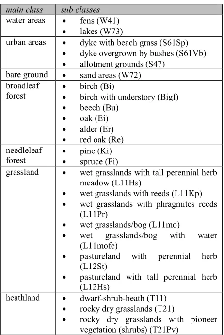
Table 3. Overview of the classes analyzed

The data was processed using the GAMMA software. 5 m was chosen as spatial resolution to fit the RapidEye data and to minimize the influence of speckle. Furthermore the Lee Sigma speckle filter was applied to the data. For every test site a TerraSAR X high resolution spotlight image was acquired.

As reference data the German biotope and land use map (Biotop und Landnutzungskartierung (BNTK)) is used. Seven main classes, as extracted from the BNTK, are used in the study. These classes are water areas, urban areas, bare ground, broadleaf forest, needleleaf forest, grassland and heathland. The seven classes are further divided into 24 subclasses (Table 3).

+' , -

. %

A detailed knowledge about the classes and features is essential for the success of the classification. The use of inadequate and redundant features during the classification process may lead to poor classification accuracy. The goal is to create a processing chain for the selection of features for all classes with the highest probability of an accurate classification.

classification is already performed and the relations between different objects of a certain class can be analyzed. Examples for relational features are distances between different classes or the distribution of these classes. Hence, the remaining feature categories were: spectral information, backscatter information (SAR), vegetation indices, texture, spectral transformations and geometric features.

+'& /

For the RapidEye data the spectral information were analyzed. Furthermore vegetation indices such as the Normalized Difference Vegetation Index (NDVI), Global Environmental Monitoring Index (GEMI), Soil Adjusted Vegetation Index (SAVI) and Enhanced Vegetation Index (EVI) and one spectral transformation (Principle Components Transformation, PCA) were computed. For the TerraSAR X data the backscatter information were analyzed. For both data sets the co occurrence texture based on Haralick and geometric features were computed. The texture measures comprise Mean, Variance, Homogeneity, Contrast, Dissimilarity, Entropy, Second Moment and Correlation and the geometric features comprise Area (m²), Length (m), Width (m), Length/Width, Compactness, Elliptic Fit, Rectangular Fit, Border length (m), Shape index, Density, Main direction and Asymmetry. The features were computed based on meaningful objects. Due to a lack of space a detailed description of every feature is renounced. A pre processing of every feature set follows the generation process.

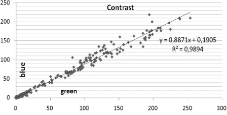
During pre processing three steps are performed: an outlier removal, data normalization and gap filling. Outliers were defined by a distance larger than three times of the standard deviation. Based on this assumption a small number of outliers were found and discarded. After the outlier removal a softmax scaling was done to fit the data in the range of [0, 1]. This is done to ensure the comparability of all features among each other. The softmax scaling is a nonlinear method but performs for small values similar to a linear method, but different to linear methods the values away from the mean are squashed exponentially. The last step of the pre processing comprises the gap filling. Due to only very few gaps in few data sets the gaps were filled by the mean value of the corresponding feature and class. Subsequently a regression analysis is performed to remove redundant information. This regression analysis is supported by a hypothesis testing using the t Test. Only if both lead to a significant measurement the tested feature is discarded. Figure 2 shows an example of a discarded feature. Figure 2 shows the regression of the texture measurement contrast computed using the blue and green band of RapidEye. The correlation is very high (R² = 0.99) and also the t Test leads to a very high value of 0.49.

Figure 2. Regression analysis example

This analysis is performed for all features. The reason why a regression analysis and a t Test are used is because only one may lead to wrong conclusions. For example the blue, green and red RapidEye bands contain very high correlation values and may be discarded. By incorporating the t Test it shows differences between the blue, green and red RapidEye bands, so that they were used for further analysis. Removed features were mainly redundant texture measurements and geometric features. These results are strongly related to the selected test sites and the analyzed classes. The analyzed vegetation classes show very high correlation for the geometric features. This is because the vegetation classes consist of very few and small irregular objects. Urban classes may show a quite different behavior.

+') 0 0

For separability analysis and feature selection in image classification the best measure should be the Bayes error. But a minimization of the Bayes error cannot be directly performed. Based on these problem alternative measurements related to the Bayes error are proposed in the literature. These criteria can be divided into three categories: 1. probabilistic distance, 2. divergence and 3. correlation based (Guo, 2008).

For this study one criterion was selected from each category and was used in the feature selection process. Under the assumption of a normal distribution of the analyzed features the following criteria can be used for feature selection. For the probabilistic distance category the Jeffries Matusita distance was chosen. The Jeffries Matusita distance is based on the Bhattacharyya distance (Bhattacharyya, 1943). For one feature and two classes the Bhattacharyya distance is given by:

=

1

8

mi

mj

2 2

σi2+ σj2

+

1

2

ln[

σi2+ σj2

2σiσj

(1)

where mi and mj are the mean values and σi and σj are the

variance values of the two feature distributions. The Bhattacharyya distance theoretically produces an infinite value range. To get a better comparison of the resulting values the Jeffries Matusita distance was used which has a finite dynamic range between 0 and 2 and is given by:

2 1

(2)

The best separability between the two analyzed classes for one feature is indicated by J = 2. The lower J becomes the worse is the separability of the classes (Nussbaum & Menz, 2008).

The divergence used in this study is based on a form of the Kullback Leibler distance (Kullback & Leibler, 1951). Similar to the Jeffries Matusita distance there is an assumption of a normal distribution of the analyzed features for the divergence. The divergence is given by:

σj2 σi2

σi2 σj2

2

m

i

m

j

i² j²

The divergence thus depends on the means and the variances. Based on this the divergence can provide large values even if the mean values of both distributions are equal. Similar to the Bhattacharyya distance for dij the resulting values are not easy to interpret. To overcome this problem the transformed divergence was used. The transformed divergence is given by:

2 1

(4)

The transformed divergence has similar to the Jeffries Matusita distance a finite dynamic range between 0 and 2. The third separability measurement was a simple correlation for all features between all classes. Additionally to the three separability measurements box plots were created for all features.

1'

".

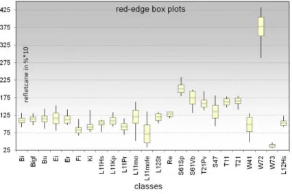
Based on the remaining features and for the 24 selected classes box plots were generated for a visual separability analysis. The box plots are very useful for a first analysis of the discrimination power of every feature. Figure 3 shows for example the discrimination ability between the broadleaf and needleleaf forest of the red edge band. Furthermore the heathland classes and urban areas can by clearly separated from the rest of the classes by using the red edge information of the RapidEye.

Figure 3. red edge box plots.

The visual comparison is followed by the evaluation of the separability measurements introduced in the previous chapter. For all features and class combinations the Jeffries Matusita distance, transformed divergence and correlation are computed (Figure 4). For every class a feature ranking was created using the separability values. The highest separability value comes first and will be integrated in the classification design. For the Jeffries Matusita distance and the transformed divergence values higher than 1.9 were interpreted as very good separability and values between 1.5 and 1.9 as good separability. For the correlation then lowest values provide the best separability.

To avoid selecting correlated features a cross correlation between the features is performed. This is necessary because

for example two features (x1 and x2) with very high

separability value are able to separate between class c1 and c2

but are not able to separate between c1 and c3, while another

feature (x3) with a lower separability value is not able to

separate between c1 and c2 but between c1 and c3. By only

using the separability values x1 and x2 were chosen and x3

would be discarded. By applying a cross correlation the described problem can be circumvented. For the cross correlation a class separability measurement (e.g. transformed divergence) is for one class ranked in descending order and the best feature with the highest transformed divergence is chosen. To select the second best features the cross correlation between the already chosen feature and each of the remaining features is computed. This means, for the selection of the next feature not only the transformed divergence but also the correlation with the already chosen feature is taken into account. This step then can be performed until the desired number of features is selected.

Figure 4. Extract of the red edge transformed divergence for the tree species classes against all classes

Afterwards the chosen features are integrated into an object and rule based classification system. For all classes thresholds for the selected features are defined. At this point the processing lacks an adequate degree of automation. This problem is the focus of current studies.

2' ! $!." ( $

The presented work shows a workflow for feature selection from high resolution remote sensing data for biotope mapping. The method can help to select suitable features for different land cover and biotope type classification approaches.

Nevertheless some limitations related to the proposed workflow should be noted. The results shown here are strongly related to the underlying objects and the existing classes in the test areas. By changing the objects sizes the feature values also change. Larger objects become spectrally more averaged but may consist of different land cover classes. A larger forest object for example can consist of shadow areas, bare ground and vegetation (trees). Small objects should hold only pure land cover classes. This leads

Bi Bu Ei Er Fi Ki

Bi 0

Bu 0.08226048 0

Ei 0.40192408 0.18092068 0 Er 0.12433847 0.02092664 0.07741988 0 Fi 1.67694489 1.69951093 1.54712234 1.58379474 0 Ki 1.10038908 1.23273755 1.16610148 1.10791623 0.37691215 0 L11Hs 0.40749204 0.70711959 0.97555382 0.68767807 1.34569321 0.51003799 L11Kp 0.08178753 0.11647281 0.18079386 0.07483325 1.34022444 0.7450641 L11Pr 0.97505079 1.04595416 0.85338583 0.87615351 0.3341652 0.02883806 L11mo 0.76654814 0.4176707 0.04359587 0.24589408 1.68465085 1.4210318 L11mofe 1.79920749 1.66532502 0.91493489 1.38482091 0.86806643 1.17814701 L12St 0.32541597 0.08007912 0.13941074 0.07588436 1.79671531 1.46201429 Re 1.03430747 0.62835003 0.72859371 0.65876105 1.98512616 1.90773828

S61Sp 1.99999969 1.99996545 1.99543317 1.99968362 2 1.99999999

S61Vb 1.99327909 1.94091244 1.50512491 1.84464776 1.99979537 1.9993745

T21Pv 1.97818986 1.89360813 1.61837456 1.81534107 1.99978768 1.998893

S47 1.41071859 0.9425054 0.33288228 0.70479807 1.93319708 1.84733103

T11 1.99251131 1.95432858 1.80979943 1.91622441 1.99997029 1.99978245

T21 1.99834884 1.9859518 1.9222025 1.97102811 1.99999724 1.9999725

W41 1.09036264 0.93700543 0.35415997 0.6518061 0.79656283 0.63297645

W72 2 2 2 2 2 2

W73 2 2 2 2 1.99975668 1.99999773

to the conclusion that the segmentation is a very important step with a high impact on the following statistical results.

Moreover the proposed method assumes for all features and classes a normal distribution. This is not always true and also has an impact on the results. A comparison between the distribution of the features and the resulting values showed that the Jeffries Matusita distance is more sensitive for not normal distributed data than the transformed divergence.

In our ongoing studies, the investigations are extended to unconsidered features. Especially relational features will be investigated. Furthermore additional classification approaches like random forest (RF) and support vector machines (SVMs) will be tested.

3'

$!

Bhattacharyya, A. A., 1943. On a measure of divergence between two statistical populations defined by their probability distributions. Calcutta Math. Soc. 35, pp. 99–110.

Bock, M., Xofis, P., Mitchley, J., Rossner, G. & Wissen, M., 2005. Object oriented methods for habitat mapping at multiple scales – Case studies from Northern Germany and Wye Downs, UK. Journal of Nature Conservation, 13, pp. 75 89.

Guo, B.; Damper, R.; Gunn, S. R. & Nelson, J., 2008 A fast separability based feature selection method for high dimensional remotely sensed image classification. Pattern Recognition, 41, pp. 1653 1662.

Kullback S. & Liebler R.A., 1951. On information and sufficiency. Annals of Mathematical Statistics, 22, pp. 79–86.

Nussbaum, S. & Menz, G. 2008. Object Based Image Analysis and Treaty Verification New Approaches in Remote Sensing – Applied to Nuclear Facilities in Iran, Springer, pp. 85 116.

Qiu, L., Gao, T., Gunnarsson, A., Hammer, M. & von Bothmer, R. 2010. A methodological study of biotope mapping in nature conservation . Urban Forestry & Urban Greening 9, pp. 161 166.

Sukopp, H. & Weiler, S. 1988. Biotope Mapping and Nature Conservation Strategies in Urban Areas of the Federal Republic of Germany. Landscape and Urban Planning, 15, pp. 39 58.

4'

! $

.

% , $