TOPOGRAPHIC CORRECTION MODULE AT STORM (TC@STORM)
K. Zakšek a,*, K. Čotar b, T. Veljanovski c, P. Pehani c, K. Oštir b,c
a University of Hamburg, CEN, Institute of Geophysics, Bundesstr. 55, 20146 Hamburg, Germany – [email protected]
b Slovenian Centre of Excellence for Space Sciences and Technologies (SPACE-SI), Aškerčeva cesta 12, SI-1000 Ljubljana, Slovenia – [email protected]
c Research Centre of the Slovenian Academy of Sciences and Arts, Novi trg 2, SI-1000 Ljubljana, Slovenia – (tatjana.veljanovski, peter.pehani, kristof.ostir)@zrc-sazu.si
KEY WORDS: Topographic Correction, Complex Terrain, Shadow Detection, Solar Irradiance, Sky-view Factor, Validation
ABSTRACT:
Different solar position in combination with terrain slope and aspect result in different illumination of inclined surfaces. Therefore, the retrieved satellite data cannot be accurately transformed to the spectral reflectance, which depends only on the land cover. The topographic correction should remove this effect and enable further automatic processing of higher level products. The topographic correction TC@STORM was developed as a module within the SPACE-SI automatic near-real-time image processing chain STORM. It combines physical approach with the standard Minnaert method. The total irradiance is modelled as a three-component irradiance: direct (dependent on incidence angle, sun zenith angle and slope), diffuse from the sky (dependent mainly on sky-view factor), and diffuse reflected from the terrain (dependent on sky-view factor and albedo). For computation of diffuse irradiation from the sky we assume an anisotropic brightness of the sky. We iteratively estimate a linear combination from 10 different models, to provide the best results. Dependent on the data resolution, we mask shades based on radiometric (image) or geometric properties. The method was tested on RapidEye, Landsat 8, and PROBA-V data. Final results of the correction were evaluated and statistically validated based on various topography settings and land cover classes. Images show great improvements in shaded areas.
* Corresponding author
1. INTRODUCTION
Data retrieved by satellite instruments depend on natural and technological circumstances. Radiometric corrections are used to account for different effects prior to the application of image interpretation. They include meteorological or atmospheric bias removal, fading the consequences of the geometry of the recording, and account for the Sun lighting and the formation of the terrain morphology. Once such radiometric processing is done, a retrieval of surface characteristics is possible. But even such a simple parameter as surface reflectance is still very challenging to retrieve in complex terrain. Slope, aspect and nearby topographic features can significantly alter the insolation received by a target and thus the radiance measured by a sensor above it (Hantson and Chuvieco, 2011; Vanonckelen et al., 2013). The most challenging is the retrieval of surface reflectance in shaded areas (Adeline et al., 2013; Dare, 2005; Oliphant et al., 2003).
Topographic correction has been gaining importance since the early 1980s through the development of IT infrastructure and photometric techniques (Cavayas, 1987; Gu and Gillespie, 1998; Justice et al., 1981; Minnaert, 1941; Riaño et al., 2003; Soenen et al., 2005; Teillet et al., 1982). A comparison between these methods was made by Hantson et al. (2011), who concluded that the best results are obtained using C-correction and empiric-statistic correction method. Some of these methods were further modified to account for more physical background (Richter, 1998; Schulmann et al., 2015).
This contribution describes the topographic correction TC@STORM that was developed as one of pre-processing modules within the automatic near real-time-image processing chain STORM. The processing chain STORM was developed
by the Slovenian Centre of Excellence for Space Sciences and Technologies (SPACE-SI), individual subtasks were developed by the Research Centre of the Slovenian Academy of Sciences and Arts. For details of the processing chain STORM see article titled Automatic Near-Real-Time Image Processing Chain for Very High Resolution Optical Satellite Data by K. Oštir et al., published on the same ISRSE36 conference.
TC@STORM has a physical approach to topographic correction. We focused on the diffuse part of irradiation. This was in previous approaches mostly modelled as an isotopic component or a sum of the isotopic and the circumsolar component. We propose an anisotropic diffuse irradiation model that has been already used for terrain visualization purposes (Zakšek et al., 2012). This model is described in section 2. The visual examples and statistical effectiveness of the proposed method is described in section 3 and results are discussed in section 4.
2. THEORETICAL BACKGROUND
TC@STORM combines physical approach to topographic correction with Minnaert method (Minnaert, 1941). The total irradiance is modelled as three-component irradiance: direct, diffuse from the sky, and diffuse reflected irradiation from the terrain.
2.1 Ratio between direct and diffuse irradiation
atmosphere solar irradiation into diffuse and direct part. The ratio between them depends on the circumstances in the atmosphere and the wavelength.
Using a radiative transfer model, we created a look-up-table (LUT) for this ratio. It depends on wavelength and elevation, the solar zenith angle and atmospheric conditions. LUT has a resolution of 1000 m for elevation, 15° for solar zenith angle, 1 nm for wavelength. According to the season we used one of the four standard atmosphere models (tropical, mid-latitude summer / winter and US 1976 standard model). In the end, the most appropriate value was interpolated from the LUT.
2.2 Direct irradiation and mask of shades estimation The influence of direct solar irradiation is straightforward to model. It depends on the incidence angle of the solar rays on terrain. If the incidence angle is larger than 90°, the terrain is in its own hill-shade. It is also possible that the horizon is higher than the Sun. Then a point is in a cast shade (behind an obstacle blocking the Sun) although the terrain might not be oriented away from the Sun.
The estimation of mask of shades is very important, because the shaded areas do not receive any direct solar irradiation. The mask of shades can be estimated using two approaches: using geometry or using radiometric values of data. Decision which approach to use was in our case based on the spatial resolution of data: satellite images might have resolutions even below 1 m, but topographical data for large areas rarely have resolutions finer than 10 m. In addition, topographical data cannot explain shades caused by the vegetation or urban objects. For that we would need an accurate digital surface model (DSM) and not a digital elevation model (DEM).
TC@STORM thus estimates mask of shades based on geometry if the resolution of data is greater than 30 m, otherwise the radiometric approach is used. As the geometric estimation of shades is straightforward we describe here only the radiometric shade estimation. This is based on histogram thresholding of the near-infrared (NIR) band. This band was chosen as it is present on most of high resolution satellite systems. In addition NIR band is less affected by scattering in the atmosphere, thus the ratio between direct and diffuse irradiance is strongly in favour to the first one. This results in shades having a stronger contrast in NIR than in visible spectrum.
Histogram thresholding is performed with Otsu’s algorithm (Otsu, 1979) which separates all pixels of the atmospherically corrected datasets into shaded areas or areas exposed to sun. However, very often water bodies are erroneously identified as shades as well. Thus, we try to mask all water bodies before we mask the shades. The water bodies are masked based on the spectral response of the water: it has its peak in the spectrum of green band (G) and then the signal drops over red band (R) to NIR band. Such mask is very successful over bodies with clear water but it can fail over turbid water. Thus we first define clear water pixels based on the ratio between G and NIR bands. Using region grow we are able to extend this mask also over turbid water pixels.
2.3 Diffuse irradiation and sky-view factor estimation The diffuse irradiance falling onto an object from the sky depends on the portion of sky visible from this object. We express this value with the sky-view factor. We assumed an anisotropic brightness of the sky. The anisotropy effect was parameterized by the angular distance of a point in the sky from the sun and the minimal brightness of the sky (Zakšek et al., 2012).
As the anisotropy depends on the usually unknown atmospheric conditions, we precomputed five different models. All of these were related to different solar positions with 30° resolution over azimuth and zenith angle. Five final models were at the end interpolated from the precomputed data according to the solar position. Fig. 1 shows both extremes (total isotopic and highly anisotropic model) and a mild version of anisotropy.
Figure 1. Examples of sky-view factor models (North-East of Slovenia, area of 15×10 km) with three different levels of anisotropy: isotropic (above), low anisotropic (middle), and high anisotropic (below); solar azimuth equals 135°and solar
zenith angle 60°.
2.4 Two models of irradiance at surface
the ground, which also has the characteristics of diffuse irradiance. We combined all the partial irradiances into two different irradiance models. Both try to model the ratio between irradiance at an inclined surface and irradiance at a horizontal surface.
The first model is built on assumption that we can model the total irradiance at both surfaces. Then we can define the following ratio r (1):
(1)
where p – ratio between the direct and total irradiance i – solar incidence angle on terrain
z – solar zenith angle svf – sky-view factor
The second model assumes that we can model separately direct and diffuse irradiance at both surfaces. Then we can define the following ratio r (2):
(2)
In the end, we iteratively estimated a model having the lowest correlation between the simulated illumination and the normalized results (see the following section 2.5).
Natural surfaces do not all have properties of a perfect Lambertian surface, thus the reflected irradiance is also affected by the reflective properties of the surface described by the bidirectional reflectance distribution function (BRDF). In the proposed method we simplify the theory behind BRDF by advancing the Minnaert method; instead of using ratio between the cosines of solar incidence angle and solar zenith angle, we here used expressions defined in Eqs. 1 and 2. Thus the reflectance after the final correction is defined as:
ρH = ρT / rK (3)
where K – Minnaert coefficient
ρT – reflectance observed over sloped terrain
ρH – reflectance equal to the horizontal surface.
2.5 Choosing the optimal model with simultaneous estimation of Minnaert coefficients
Expressions in Eqs. 1 and 2 describe the ratio between irradiance at the inclined and horizontal surface. According to the theory of Minnaert method, the logarithm of these values is linearly correlated to the logarithm of uncorrected satellite data; let’s name this correlation corr1. In this process coefficient K is defined as slope in linear regression between those two logarithmic values. After applying the correction it is expected that the correlation is reduced to ~0; let’s name this correlation corr2. Since the exact conditions in the atmosphere are not known, the choice of the optimal predefined models of diffuse irradiance is difficult. Therefore, we make a use of the calculated values corr1 and corr2. The first one should be as large as possible and the second one as close to zero as possible. This means that the ratio corr1 / corr2 should be as large as possible.
With this statistical selection condition in mind, we apply the calibration of Minnaert model for all five diffuse irradiation models and for both surface irradiance models (Eqs. 1 and 2).
From 10 models we select the one having the highest ratio corr1 / corr2. This is done for each band separately.
We have tested this calibration also separately for different land cover classes, because different classes have different BRDFs. For such an implementation, however, it is necessary to have a very detailed land cover map for the whole processed area, which in general is difficult to obtain for large areas. In all tests performed the Minnaert coefficients over different land cover classes did not show a significant variation, therefore we decided to apply this calibration without considering the land cover data.
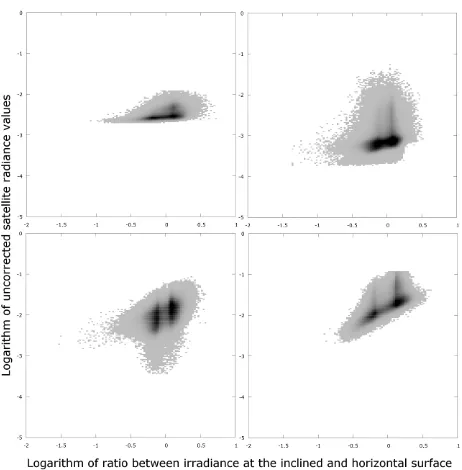
Figure 2. Density scatter plots of the reflectance values of different spectral bands that are used in the linear regression
when determining optimal model and coefficient K.
3. VISUAL AND STATISTICAL VALIDATION In this section we focus on the evaluation of the capacity of the proposed topographic correction method. The efficiency and success of any process is most intuitive evaluated through: (1) the sensitivity/robustness analysis of the algorithm in relation to parameters and selected decisions involved in the process, (2) direct analysis of the effects correction has achieved and (3) comparison of the results with other topographic correction methods.
impression is that proposed method over-performs traditional models as Cosine model, Minnaert correction, C-Factor as well as their improved versions such as SCS model.
3.1 Defining validation measures
In order to understand the results of the proposed correction method we have tested it on three datasets of different spatial and spectral resolutions, covering the area of Slovenia and abroad. We have applied full-scene processing to six PROBA-V, eleven Landsat 8 and fourteen RapidEye images (Table 1). Selected images are mainly cloud-free and from different seasons to get insight into how a variable Sun position and related illumination affect the correction process.
Sensor No. of
images resolution Spatial resolution Spectral
PROBA-V 6 100 m 4 bands:
Table 1. Overview of data used in the topographic correction study and validation.
The multi-sided validation proved beneficial to the understanding of topographic correction performance. For each image we have inspected correction’s overall visual performance and integrity, and a range of statistical measures. With statistical analysis we aimed to verify general assumptions that correspond to the purpose of applying topographic correction in remote sensing image pre-processing. Statistical analyses include correction’s performance over different terrain settings (slope, aspect, land cover) for each sensor and spectral band under consideration. In addition, we have inspected relations between incidence angle and reflectance, relations between image acquisition date within a year (day-of-year, DOY) and reflectance over spectral bands and land cover classes. For the evaluation of the model’s key parameters we have inspected relation between ratio of irradiance at the inclined and horizontal surface and reflectance. To ease the interpretation of rather complex relations, their combinations and thus boundless range of representations all the statistical calculations were also displayed on corresponding plots. Due to large number of cross-relations we have tested we will focus our findings only on most representative situations: on spectral bands that are available at all the three sensors datasets (G, R and NIR spectral bands) and on land cover classes that show less ambiguity within their natural representations on the Earth surface (agriculture, broad-leaf forest, coniferous forest, mixed forest, shrub/herbaceous and barren/open, and thus omitting urban and water land cover classes).
3.2 Estimation of the best Minnaert coefficient K and its variability
Estimation of the coefficient K (described in section 2.5) can be visually supervised by a density scatter plot for every precomputed model. From those plots (Fig. 2) we can identify specific point clouds that could lead to incorrectly estimated K
value and should be removed before the linear regression step. Most obvious features in those graphs are vertical lines, representing pixels with fairly high reflectance variability at low slope angles, usually associated with barren/open ground pixels. As K values are estimated independently for every image scene and spectral band, there is notable variability between their values.
All the sensors show the same trend in the estimated K values. The lowest K values were estimated for a spectral band with the minimum wavelength (blue band). K values are gradually increasing as the band wavelength increases, and have a maximum value for the NIR band where K may reach a value of 1. For wavelengths longer than NIR band (i.e. SWIR bands) K values decreases.
3.3 Selection of the equation model
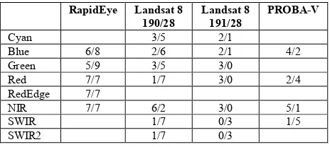
For estimation of the best value for K we are combining five different pre-calculated SVF models and two different irradiance equations, which give us 10 possible combinations for the final topographic correction model. Selection of the best possible combination is explained in section 2.5. In the validation stage we were interested in the distribution of the selected equation, however not in the distribution of the selected SVF model.
Distribution of the selected equation was studied depending on sensor type and spectral band. Results are presented in Table 2, where the left number in cell indicates the number of the images for which Eq. 1 was selected and the right number gives the
Table 2. Distribution of used irradiance equations (Eq. 1 / Eq. 2) among different sensors and spectral bands.
Results in Table 2 show clear preference for equation selection for NIR and SWIR bands of all the sensor types, however inconclusive results for other spectral bands of selected test images. Disagreement in equation selection for adjacent Landsat 8 scenes may depend on their completely different topography. Landsat 8 scene 191/28 covers the area predominant with high mountains in contrast to the scene 190/28 where hilly mountains and lowlands prevail.
The opposite situation can be observed for RapidEye data. All the images used in this study except one were captured over the hilly lands and arable lands in lowlands with no prominent mountains. From the equation distribution it is obvious that both equations can be equally used in such topographic conditions.
3.4 Incidence angle and reflectance
incidence angle. Furthermore, from the same plot we could inspect the performance of land cover separability for different spatial resolutions as the same land cover image was used for all the images. Fig. 3 shows strong correlation between reflectance and incidence angle before the correction is applied to image. After the correction reflectance values are equalized and the distribution graph is flattened out. The topographic impact varies both with wavelength and land cover and is most prevalent in NIR bands. Overcorrection can occur for steep shaded slopes with low (less than 0.2) cos(i) or for pixels with cos(i) close to 1 as shown in Fig. 3.
Figure 3. Upper images show reflectance density plot of PROBA-V NIR reflectance in broad-leaf forest land cover class
before and after topographic correction. As expected, the reflectance values are flattened out for all the cos(i) values, whereas overcorrection is evident for pixels with high cos(i).
3.5 Topographic correction and terrain characteristics The reflectance points represented in section 3.4 can also be plotted with respect to their topography settings (slope, aspect). Different solar position in combination with terrain slope and aspect result in different illumination of inclined surfaces. Therefore retrieved surface reflectance is dependent on terrain slope, aspect and land cover characteristics. To observe response of the proposed method in a multitude of different landscape occurrences (natural settings) we have analysed reflectance relative error in relation to flat-like areas conditions across aspect, slope, land cover and spectral band, respectively. To estimate the gain in the reflectance retrieval we have to observe the situation before and after the correction. For each image before and after statistics were calculated and corresponding plot was depicted.
Under the above assumption we expect that aspect and slope curves describing situation before the correction will be flattened close to zero after the correction. Results (Fig. 4) show that for the aspect this is mostly true and can be identified in all three datasets. The proposed correction especially successfully
mitigates aspect in NIR and SWIR spectrum, while in visible spectrum same effect is also present but performs far less consistently. More stable results were obtained in forest and shrub land cover classes and as the spectral band wavelength increase.
Datasets from all three sensors show the same trend in NIR spectrum, which shows most stable and consistent topographic correction results. This means that aspect in NIR spectrum is always properly neutralised, notwithstanding sensor type, spatial resolution, date of acquisition or land cover. While in SWIR spectrum correction is also highly effective, occasionally turn-overs in correction direction (over- and under corrections) can be traced. This is mainly associated with steeper slopes, while on gentle slopes such turn-overs are rare.
Regarding the slope the results do not support general assumption that reflectance values would be equalised and that distance between slope classes would be narrowed after the correction. The differences in the intensity of the slope remain present also after corrections and are not mitigated as assumed.
Figure 4. Relative errors between mean reflectance in lowlands (0-2° slope) and mean hillside reflectance for different slope
ranges (colour curves) plotted against aspect for 3 spectral bands of Landsat 8 and broad-leaf forest land cover class. Curves show successful retrieval of reflectance values for all aspect values in red and NIR band. SWIR curves show turnover
effect for higher slope values.
perfectly suited for Landsat data, where its entire spectrum is improved with respect to topographic influences. This is also valid for the only tested RapidEye image that is covering the mountainous area. While for the rest of RapidEye dataset that is covering an area of flat terrain, improvements were present mainly in NIR and RedEdge spectrum. With PROBA-V images mostly red, NIR and SWIR spectrum is improved, however, mainly for a good mitigation of aspect, still not frequently reaching the anticipated stabilisation close to zero. The morphology of the terrain thus also implicates the correction and retrieval of its share over the spectrum.
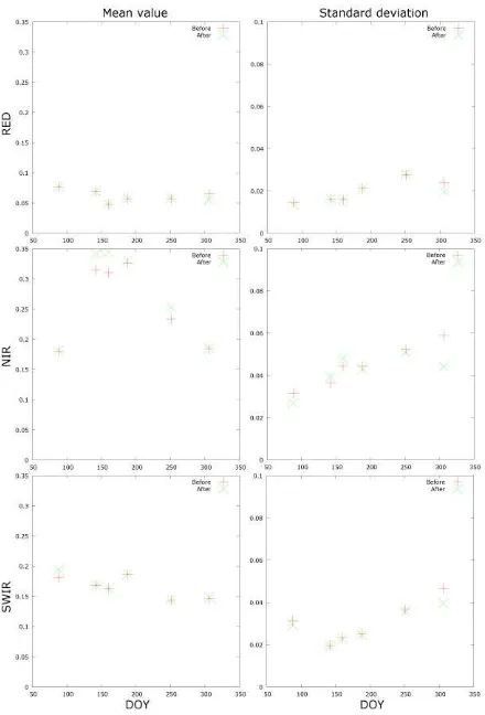
3.6 Topographic correction and the image acquisition date Reflectance mean and standard deviation before and after the topographic correction was plotted against the image acquisition date (DOY) for each spectral band and land cover class (see Fig. 5).
This gives us insight if and how topographic correction is dependent on seasonal variations and thus in addition, which spectral band and/or land cover class is more susceptible to particular illumination conditions.
Figure 5. Example of mean and standard deviation plots for PROBA-V bands and broad-leaf forest land cover class before
and after topographic correction.
As assumed, scene mean reflectance for all three datasets after correction is in general higher than before the correction in most of the tested examples. This proves that topographic correction is retrieving and increasing pixels values of shaded areas. Scene standard deviation is in general diminished, although in several cases it may increase. Increase is present
mainly in next cases: on Landsat 8 images in open and occasionally shrub land cover classes in all spectral bands, on RapidEye images NIR band exhibits some unpredictable variability, on PROBA-V images standard deviation on average is increased in all bands (least in NIR band).
In terms of mean reflectance statistics (over the scene) we can observe rather stable behaviour in spectral bands of visual spectrum (i.e. blue, green and red bands) all over the year and for all land cover classes and sensors. Slight shifts can be observed in spring and autumn season, however tested sample may be too small to derive firm conclusions. In general three types of “curve” pattern over DOY scale (starting and ending in January) can be identified: gentle sinusoidal in spectral bands of visible spectrum, expressed bell-curve in NIR bands, and flattened bell-curve (sometimes close to line) in SWIR bands. A gentle sinusoidal behaviour over the year is having slight peaks in spring and autumn imagery dates and slight valleys in summer season (winter imagery was not included in testing). On the other hand a bell-curved pattern has a peak over the summer period. This could suggest that topographic correction performs somewhat season-related in the visible bands; while having more predictable performance in the IR spectrum during summer period.
Correction strength is lowest in the visible spectrum, followed by SWIR spectrum and highest in NIR spectrum, where greater variability over DOY scale and land cover classes is also identified. Corrections are also more diverse (and do not exhibit clear pattern) in land cover classes where higher level of heterogeneity is present (agriculture, urban, mixed forest and shrub/herbaceous). Rather special case is land cover class barren/open area that in general, regardless spectral bands and sensors, receives strongest corrections. This should be due to the fact that this class mainly covers high mountain peaks, and thus steepest slopes among all land cover classes.
From corresponding standard deviation we can observe that in general standard deviation after correction decreases and that its change rate (comparing before and after image reflectance) is lower in visible spectrum and higher and more diverse in IR spectrum. It can be also observed that bigger divergences are presented in agriculture, shrub/herbaceous and all forest land cover classes.
In general the correction is strongest in infrared bands (NIR and SWIR). For example, mean retrieved reflectance in shadows for PROBA-V imagery can reach a value up to 2–3 times of mean reflectance before correction, in contrast to the visible bands where it ranges to 1–2 times.
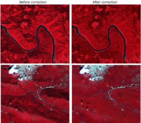
3.7 Visual inspection
Objective of topographic correction is elimination of topography illumination differences. Normalizing an image in this way changes its visual appearance so that influence of topography is extensively reduced and image appears flat. Visual control is thus mainly concerned with after-correction terrain de-shadowing appearance and overall colour (band) integrity representation (Fig. 6 and Fig. 7).
Figure 6. Final result of topographic correction in hilly area for all three sensors. Colour image is composed of NIR-R-B/G
spectral bands.
Figure 7. Close up images of correction results for RapidEye.
4. DISCUSSION AND CONCLUSIONS
The objective of this study was to test and validate the proposed topographic correction method. We have conducted a multi-sided validation in order to obtain insight into correction’s advantages and potential pitfalls regarding the topographic correction that is implemented within the processing chain STORM. Our objective was to get answers to the issues we are addressing in more detail in the following paragraphs.
What is a reasonable range of data spatial resolution for a topographic correction? This issue needs to be associated with higher level products generation and interpretation. Especially in applications where time-series or bio-physical (vegetation) indicators are involved illumination compensation becomes indispensable. Taking into account validation results we can conclude that topographic correction should always be applied to imagery of spatial resolution between 5 and up to several 10 m, as correction will appropriately affect entire spectrum (visible, NIR in SWIR). It might be less binding but still welcome for imagery of 100 m spatial resolution, where mainly IR and SWIR spectrum will be mitigated for topographic effects but thus, for example, ensuring accurate vegetation observations and analysis. When taking into account different spatial resolutions for the topographic correction it is of utmost importance to ensure appropriate and high quality digital elevation data.
How topographic correction reflects in different spectral bands? Multi-sided validation reveals that proposed correction especially successfully mitigates aspect in NIR and SWIR spectrum, while in visible spectrum is also present but may performs less consistently. Inconsistency can be attributed mainly to differences in relief morphology and land cover settings. Datasets from all the three sensors shows the same trend in the NIR spectrum, which is thus recognized as most stable and consistent in topographic correction. This means that aspect in NIR spectrum is always properly neutralised, notwithstanding sensor type, spatial resolution, and date of acquisition or land cover. While in SWIR spectrum correction is also highly effective, occasionally over or under corrections can be present. It does not mean that for sensors of higher spatial resolution imagery visible spectrum remains uncorrected, just the strength of correction is lower in comparison to IR spectrums.
How the method responds to different surface illumination situations? Study on more than 30 images acquired in different days all over the year proves that proposed method responds to all illumination conditions. Further, we can conclude that solving geometric part of Sun-terrain-sensor geometry within the correction is not problematic. The greater challenge is definition of suitable K parameter, thus selection of the appropriate calibration pixels.
What is the role of surface characteristics in the topographic correction process? Surface or land cover natural representation and how it is depicted in the satellite image may influence several decisions in topographic correction. Surface reflection or albedo (i.e. spectral properties) and surface roughness (i.e textural properties) directly address the most important parameter calculation in the correction process (the coefficient K value for Minnaert model). On the other hand, validation results reveals that in highly homogenous land cover classes the topographic correction can almost reach the theoretical assumptions (curve flattering around zero). However, as within class homogeneity is violated also correction slightly deviates from the expected scope of operation.
are still representative. It re-confirms reflectance retrieval in shadows is band dependent and increase with wavelength: on average mean shadow reflectance is increased 1.2 times in green band, 1.9 times in red band, 3.7 times in NIR and 3 times in SWIR in contrast to mean shadow reflectance before correction was applied.
To conclude, we demonstrated that proposed method successfully retrieves reflectance in complex topography conditions on datasets of different spatial and spectral resolutions. Further work will focus on the observed problems such as separation between water and shadow pixels and determining optimal model and coefficient K.
ACKNOWLEDGEMENTS
Research was partly financed by the Slovenian Research Agency project J2-6777. The research has been supported also by grants from the German Science Foundation (DFG) number ZA659/1-1. The Centre of Excellence for Space Sciences and Technologies SPACE-SI was an operation partly financed by the European Union, European Regional Development Fund, and Republic of Slovenia, Ministry of Higher Education, Science and Technology (2010–2013). Research was also partly financed by the Republic of Slovenia through the ESA PECS programme (W4000106563/14/NL/NDE).
PROBA-V data and consultancy on the use of PROBA-V data have been provided by VITO.
REFERENCES
Adeline, K.R.M., Chen, M., Briottet, X., Pang, S.K., Paparoditis, N., 2013. Shadow detection in very high spatial resolution aerial images: A comparative study. ISPRS J.
Photogramm. Remote Sens. 80, 21–38.
doi:10.1016/j.isprsjprs.2013.02.003
Cavayas, F., 1987. Modelling and Correction of Topographic Effect Using Multi-Temporal Satellite Images. Can. J. Remote Sens. 13, 49–67. doi:10.1080/07038992.1987.10855108
Dare, P.M., 2005. Shadow Analysis in High-Resolution Satellite Imagery of Urban Areas. Photogramm. Eng. Remote Sens. 71, 169–177. doi:10.14358/PERS.71.2.169
Gu, D., Gillespie, A., 1998. Topographic Normalization of Landsat TM Images of Forest Based on Subpixel Sun–Canopy– Sensor Geometry. Remote Sens. Environ. 64, 166–175. doi:10.1016/S0034-4257(97)00177-6
Hantson, S., Chuvieco, E., 2011. Evaluation of different topographic correction methods for Landsat imagery. Int. J. Appl. Earth Obs. Geoinformation 13, 691–700. doi:10.1016/j.jag.2011.05.001
Justice, C.O., WHARTON, S.W., HOLBEN, B.N., 1981. Application of digital terrain data to quantify and reduce the topographic effect on Landsat data. Int. J. Remote Sens. 2, 213– 230. doi:10.1080/01431168108948358
Minnaert, M., 1941. The reciprocity principle in lunar photometry. Astrophys. J. 93, 403. doi:10.1086/144279
Oliphant, A.J., Spronken-Smith, R.A., Sturman, A.P., Owens, I.F., 2003. Spatial Variability of Surface Radiation Fluxes in
Mountainous Terrain. J. Appl. Meteorol. 42, 113–128. doi:10.1175/1520-0450(2003)042<0113:SVOSRF>2.0.CO;2
Otsu, N., 1979. A Threshold Selection Method from Gray-Level Histograms. IEEE Trans. Syst. Man Cybern. 9, 62–66. doi:10.1109/TSMC.1979.4310076
Riaño, D., Chuvieco, E., Salas, J., Aguado, I., 2003. Assessment of different topographic corrections in Landsat-TM data for mapping vegetation types (2003). IEEE Trans. Geosci. Remote Sens. 41, 1056–1061. doi:10.1109/TGRS.2003.811693
Richter, R., 1998. Correction of satellite imagery over mountainous terrain. Appl. Opt. 37, 4004–4015. doi:10.1364/AO.37.004004
Schulmann, T., Katurji, M., Zawar-Reza, P., 2015. Seeing through shadow: Modelling surface irradiance for topographic correction of Landsat ETM+ data. ISPRS J. Photogramm. Remote Sens. 99, 14–24. doi:10.1016/j.isprsjprs.2014.10.004
Soenen, S.A., Peddle, D.R., Coburn, C.A., 2005. SCS+C: A Modified Sun-Canopy-Sensor Topographic Correction in Forested Terrain. IEEE Trans. Geosci. Remote Sens. 43, 2148– 2159. doi:10.1109/TGRS.2005.852480
Teillet, P., Guindon, B., Goodenough, D., 1982. On the slope-aspect correction of multispectral scanner data. Can. J. Remote Sens. 8, 84–106.
Vanonckelen, S., Lhermitte, S., Van Rompaey, A., 2013. The effect of atmospheric and topographic correction methods on land cover classification accuracy. Int. J. Appl. Earth Obs. Geoinformation 24, 9–21. doi:10.1016/j.jag.2013.02.003